Project: Smoothing#

Smoothing is used to reduce the impact of fluctuations such as spikes or errors.
Smoothed values deviate from actual data points, yet they encapsulate the overall behavioral trends within the dataset.
import matplotlib.pyplot as plt
import numpy as np
Data#
In this project, we will use the following Apple daily stock price data for a particular period of time.
# the opening price at the beginning of each day
open = [182.60232902746063,
 182.31272011600538,
 184.89999389648438,
 185.44000244140625,
 187.50999450683594,
 187.91000366210938,
 190.47000122070312,
 189.50999450683594,
 189.3300018310547,
 191.08999633789062,
 192.27000427246094,
 190.97999572753906,
 188.82000732421875,
 191.50999450683594,
 189.61000061035156,
 190.75999450683594,
 191.44000244140625,
 192.89999389648438,
 194.63999938964844,
 195.39999389648438,
 195.69000244140625,
 194.64999389648438]
# the closing price at the end of each day
close = [182.4924774169922,
 184.32000732421875,
 183.0500030517578,
 186.27999877929688,
 187.42999267578125,
 189.72000122070312,
 189.83999633789062,
 189.8699951171875,
 191.0399932861328,
 192.35000610351562,
 190.89999389648438,
 186.8800048828125,
 189.97999572753906,
 189.99000549316406,
 190.2899932861328,
 191.2899932861328,
 192.25,
 194.02999877929688,
 194.35000610351562,
 195.8699951171875,
 194.47999572753906,
 196.88999938964844]
# The lowest price reached during each day.
low = [181.20421623621485,
 181.86333268844692,
 182.1300048828125,
 184.6199951171875,
 186.2899932861328,
 187.3699951171875,
 189.66000366210938,
 189.17999267578125,
 189.00999450683594,
 190.9199981689453,
 190.27000427246094,
 186.6300048828125,
 188.0399932861328,
 189.10000610351562,
 189.50999450683594,
 190.6300048828125,
 189.91000366210938,
 192.52000427246094,
 193.02999877929688,
 194.8699951171875,
 194.1699981689453,
 194.13999938964844]
# The highest price reached during each day.
high = [182.82203224839753,
 184.4098817621062,
 185.08999633789062,
 187.10000610351562,
 188.3000030517578,
 190.64999389648438,
 191.10000610351562,
 190.80999755859375,
 191.9199981689453,
 192.72999572753906,
 192.82000732421875,
 191.0,
 190.5800018310547,
 193.0,
 192.25,
 192.17999267578125,
 192.57000732421875,
 194.99000549316406,
 195.32000732421875,
 196.89999389648438,
 196.5,
 196.94000244140625]
# number of days
N = len(high)
N
22
# the list of days
days = ['day_'+str(i) for i in range(1, N+1)]
days
['day_1',
 'day_2',
 'day_3',
 'day_4',
 'day_5',
 'day_6',
 'day_7',
 'day_8',
 'day_9',
 'day_10',
 'day_11',
 'day_12',
 'day_13',
 'day_14',
 'day_15',
 'day_16',
 'day_17',
 'day_18',
 'day_19',
 'day_20',
 'day_21',
 'day_22']
Stock Behavior#
The list indicating the behavior of stock prices as Increasing, Decreasing, or Flat.
change = []
for i in range(N):
    if close[i] > open[i]:
        change.append('Inc')
    elif close[i] < open[i]:
        change.append('Dec')
    else:
        change.append('Flat')

change
['Dec',
 'Inc',
 'Dec',
 'Inc',
 'Dec',
 'Inc',
 'Dec',
 'Inc',
 'Inc',
 'Inc',
 'Dec',
 'Dec',
 'Inc',
 'Dec',
 'Inc',
 'Inc',
 'Inc',
 'Inc',
 'Dec',
 'Inc',
 'Dec',
 'Inc']
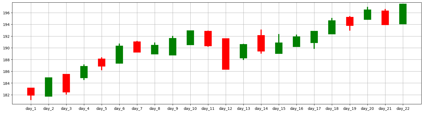
Candlestick#
Candlesticks are used to identify patterns in stock data.
Red color indicates a decrease, while green color indicates an increase.
The lower and upper parts of the rectangle represent the opening and closing values.
The lower and upper parts of the line represent the lowest and highest values.
plt.figure(figsize=(20,5))

for i in range(N):

    if change[i] == 'Inc':
        col = 'green'
    elif change[i] == 'Dec':
        col = 'red'
    else:
        col = 'blue'

    plt.plot([days[i],days[i]],[open[i], close[i]], c=col, linewidth=20)
    plt.plot([days[i],days[i]],[low[i], high[i]], c=col, linewidth=3)

plt.grid()
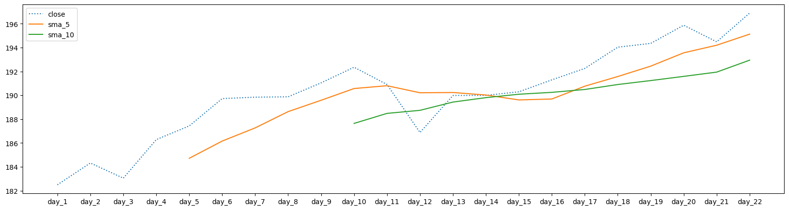
SMA#
Simple Moving Average
SMA calculates the average value within a chosen time frame.
All values are weighted equally, without distinction between old and new data points.
\(SMA_k\) is represents the sequence of the average of k consecutive values of the original data
Formula: \(\displaystyle SMA_k = \frac{x_n+x_{n+1}+x_{n+2}+...+x_{n+k-1}}{k}\)
For the first k−1 values, there is no average value because there are fewer than k values available.
The first k−1 values of \(SMA_k\) are NaN (Not a Number).
def sma(seq, k):
    sma_list = [np.nan]*(k-1)
    for n in range(len(seq)-k+1):
        sma_list.append(sum(seq[n:n+k])/k)
    return sma_list
len(sma(close, 3))
22
plt.figure(figsize=(20,5))
plt.plot(days, close, label='close', linestyle='dotted')
plt.plot(sma(close, 5), label='sma_5')
plt.plot(sma(close, 10), label='sma_10')
plt.legend();
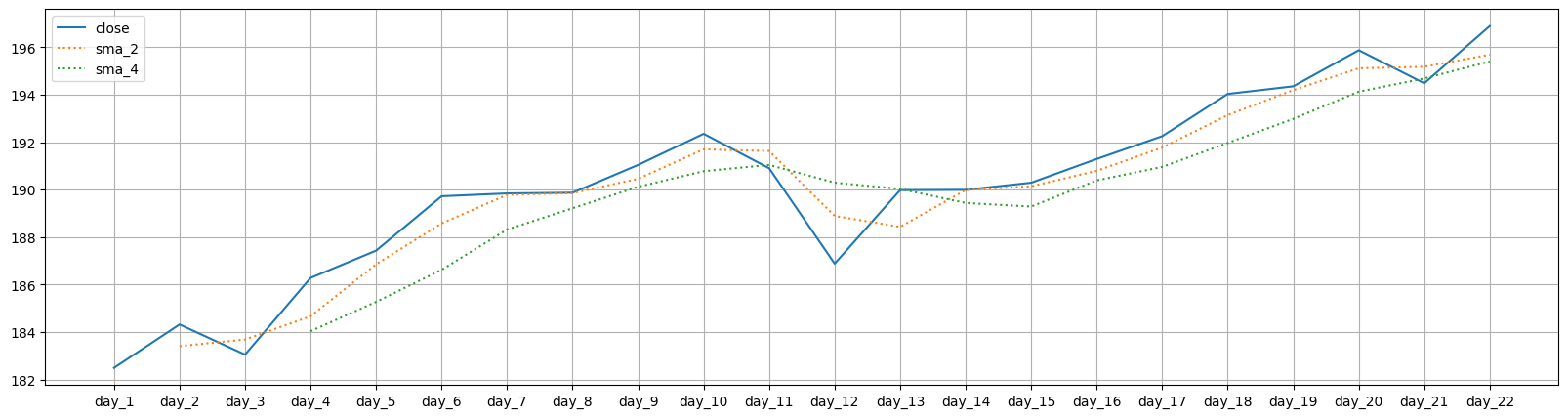
Moving Average Signals#
A buy signal happens when the shorter-term moving average (MA) crosses above the longer-term MA, indicating an upward trend shift known as a “golden cross”.
A sell signal occurs when the shorter-term moving average (MA) crosses below the longer-term MA, signaling a downward trend shift known as a “death cross”.
Reference: www.investopedia.com
There are two intersections between the \(SMA_2\) and \(SMA_4\) graphs.
plt.figure(figsize=(20,5))
plt.plot(days, close, label='close')
plt.plot(sma(close, 2), label='sma_2', linestyle='dotted')
plt.plot(sma(close, 4), label='sma_4', linestyle='dotted')
plt.xticks(range(len(days)), days)
plt.grid()
plt.legend();
for i in range(len(close)-1):
    if (sma(close, 2)[i] > sma(close, 4)[i]) & (sma(close, 2)[i+1] < sma(close, 4)[i+1]):
        print(f'Death cross  : day_{i+1} -- day_{i+2}')
    if (sma(close, 2)[i] < sma(close, 4)[i]) & (sma(close, 2)[i+1] > sma(close, 4)[i+1]):
        print(f'Golden Crsoss: day_{i+1} -- day_{i+2}')
Death cross  : day_11 -- day_12
Golden Crsoss: day_13 -- day_14
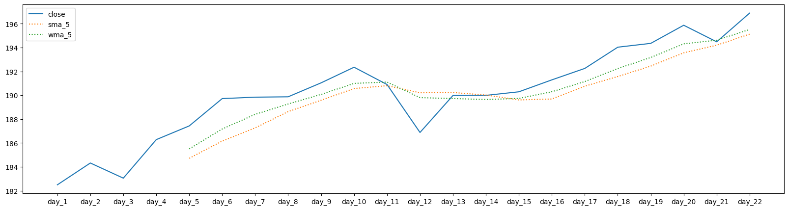
WMA#
Weighted Moving Average
WMA computes the weighted average value over a specified time period.
Unlike SMA, the weights assigned to values may vary, with newer data points potentially carrying more significance than older ones.
The influence of new points surpasses that of old points.
\(\displaystyle WMA_k = \frac{x_n + 2x_{n+1} + 3x_{n+2} + ... + kx_{n+k-1}}{1 + 2 + ... + k}\)
def wma(seq, k):
    wma_list = [np.nan]*(k-1)
    for n in range(len(seq)-k+1):

        num = 0
        for i in range(k):
            num += (i+1)*seq[n+i]

        den = sum(range(1,k+1))
        wma_list.append(num/den)
    return wma_list
plt.figure(figsize=(20,5))
plt.plot(days, close, label='close')
plt.plot(sma(close, 5), label='sma_5', linestyle='dotted')
plt.plot(wma(close, 5), label='wma_5', linestyle='dotted')
plt.legend();
EWA#
Exponential Weighted Average
\( s_0 = x_0 \)
\( s_t = \alpha x_t +(1-\alpha) s_{t-1}\) for \(t>0\)
where \(\alpha\) is between 0 and 1.
\( s_0 = x_0 \)
\( s_1 = \alpha x_1 + (1-\alpha)s_0 = \alpha x_1 + (1-\alpha)x_0\)
\( s_2 = \alpha x_2 + (1-\alpha)s_1 = \alpha x_2 + (1-\alpha)(\alpha x_1 + (1-\alpha)x_0) = \alpha x_2 + (1-\alpha)\alpha x_1 + (1-\alpha)^2x_0\)
def ewa(seq, alpha):
    s = [seq[0]]
    for n in range(1,len(seq)):
        s.append(alpha*seq[n]+(1-alpha)*s[-1])
    return s
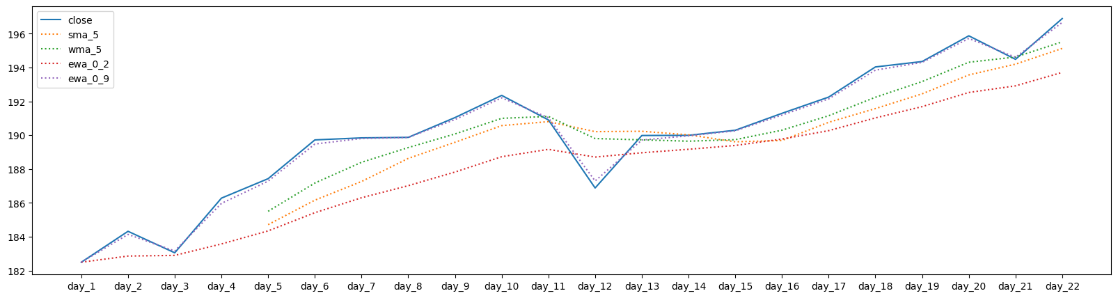
plt.figure(figsize=(20,5))
plt.plot(days, close, label='close')
plt.plot(sma(close, 5), label='sma_5', linestyle='dotted')
plt.plot(wma(close, 5), label='wma_5', linestyle='dotted')
plt.plot(ewa(close, 0.2), label='ewa_0_2', linestyle='dotted')
plt.plot(ewa(close, 0.9), label='ewa_0_9', linestyle='dotted')
plt.legend();
AEWA#
Adjusted Exponential Weighted Average
Similar to WMA, but with different weights.
It is calculated using weights: \(1, (1-\alpha), (1-\alpha)^2, (1-\alpha)^3, ...\)
\(\displaystyle AEWA_k = \frac{(1-\alpha)^{k-1}x_n + (1-\alpha)^{k-2}x_{n+1} + ... +(1-\alpha)x_{n+k-2} + x_{n+k-1}}{ (1-\alpha)^{k-1}+(1-\alpha)^{k-2}+...+(1-\alpha)+1}\)
Example If k = 5,
\(\displaystyle AEWA_5 = \frac{(1-\alpha)^{4}x_n +(1-\alpha)^{3}x_{n+1}+(1-\alpha)^{2}x_{n+2}+(1-\alpha)x_{n+3}+x_{n+4}} { (1-\alpha)^{4}+(1-\alpha)^{3}+(1-\alpha)^{2}+(1-\alpha)+1}\)
def aewa(seq, k, alpha):
    aewa_list = [np.nan]*(k-1)
    for n in range(len(seq)-k+1):

        num = 0
        for i in range(k):
            num += seq[n+i]*(1-alpha)**(k-i-1)

        den = sum([(1-alpha)**(k-i) for i in range(1,k+1)])
        aewa_list.append(num/den)
    return aewa_list
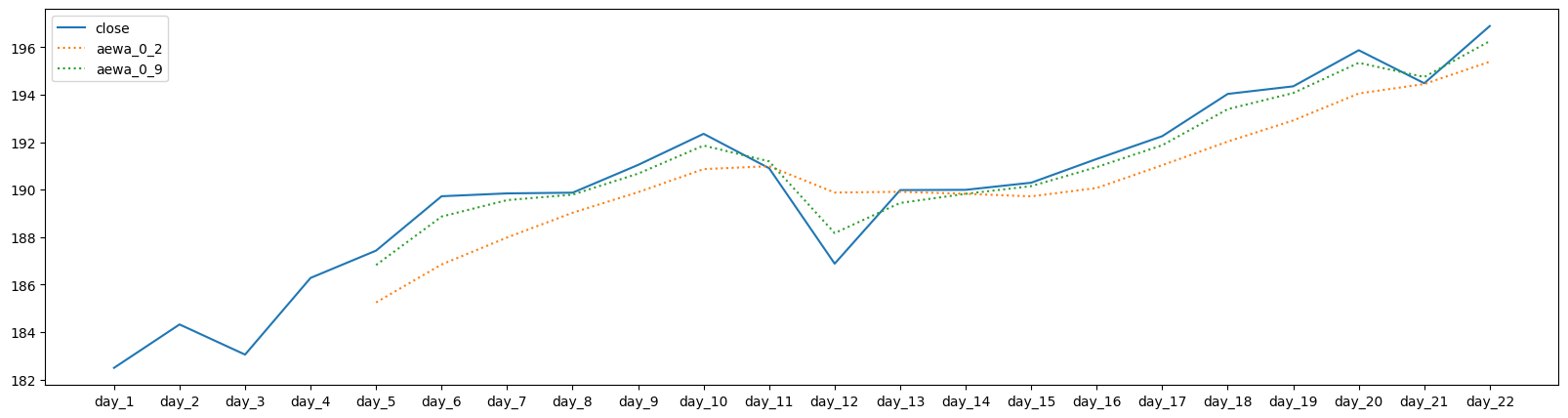
plt.figure(figsize=(20,5))
plt.plot(days, close, label='close')
plt.plot(aewa(close, 5, 0.2), label='aewa_0_2', linestyle='dotted')
plt.plot(aewa(close, 5, 0.7), label='aewa_0_9', linestyle='dotted')
plt.legend();
Future work#
Similar analyses can be conducted with additional data. To import stock data, you can use the yfinance package.
Install it using
!pip3 install yfinance.Use the stock symbol to import historical price data.
For example, the symbol for Apple is AAPL, which is used in the following code to import data from ‘1/1/2010’ to ‘12/31/2023’.
import yfinance as yf
apple_data = yf.Ticker('AAPL').history(start='2010-1-1', end='2023-12-31')
apple = apple_data['Close'].tolist()
len(apple)
3522
The list apple has a length of 3,522.
You can use 50 and 200 periods for SMA to identify potential golden and death crosses.