Isolation Forest

• Isolation Forest determines the outliers in a data.

• It returns -1 for outliers and 1 for inliers.

Method

1. For each split, a random feature is chosen, and a value between the feature’s minimum and maximum is selected.

2. This process is recursively applied to split all the samples.

3. The average number of splits required to isolate a sample, across an ensemble of trees, is called the normality measure.

4. Outliers require fewer splits to be isolated, so their normality measure is smaller compared to inliers.

Example

import numpy as np
import pandas as pd
import matplotlib.pyplot as plt

np.random.seed(0)
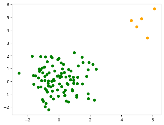
data1 = np.random.normal(size=(100,2)) 
data2 = np.random.normal(loc=5, size=(5,2)) 

plt.scatter(data1[:,0], data1[:,1], c='g')
plt.scatter(data2[:,0], data2[:,1], c='orange');

X = np.vstack([data1, data2])
X.shape

(105, 2)

from sklearn.ensemble import IsolationForest
clf = IsolationForest(random_state=0)
clf.fit(X)

IsolationForest(random_state=0)

In a Jupyter environment, please rerun this cell to show the HTML representation or trust the notebook.
On GitHub, the HTML representation is unable to render, please try loading this page with nbviewer.org.

predictions = clf.predict(X)

from collections import Counter
Counter(predictions)

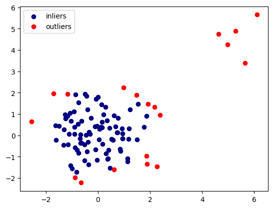
Counter({1: 86, -1: 19})

inliers = X[predictions == 1]
outliers = X[predictions == -1]

plt.scatter(inliers[:,0],  inliers[:,1], c='navy', label='inliers')
plt.scatter(outliers[:,0], outliers[:,1], c='red', label='outliers')
plt.legend();

# Average anomaly score of X of the base classifiers.
clf.decision_function(X)

array([ 0.02312107, -0.07530189, -0.00456119,  0.08818199,  0.10160557,
        0.03584609,  0.09932992,  0.10090331,  0.02923225,  0.06804123,
       -0.13577388,  0.06699841, -0.0833435 ,  0.10420727,  0.01350973,
        0.10994401, -0.04227785,  0.10242173,  0.0264283 ,  0.10040098,
        0.0151073 , -0.0670491 ,  0.099482  ,  0.08273729,  0.0265511 ,
        0.10860788,  0.05392592,  0.10279865,  0.1061506 ,  0.10184561,
        0.10456211,  0.00265429,  0.08428358,  0.05317393,  0.10700338,
        0.09905358,  0.01340571,  0.07944365,  0.0883821 ,  0.09969933,
        0.08251061,  0.00280412, -0.02215977,  0.05953927,  0.06230175,
        0.05684366,  0.07385389,  0.08762826,  0.02967877,  0.11119139,
       -0.0279606 ,  0.0631309 , -0.0028059 ,  0.08704871, -0.00195314,
        0.02053852,  0.01973971,  0.08760846,  0.08791454,  0.07102515,
        0.05769716,  0.03604464,  0.11005366,  0.02451027,  0.09327784,
        0.10999299,  0.10801372,  0.09913288,  0.08961188,  0.05973061,
        0.05980827,  0.09840725, -0.06712055,  0.06673036,  0.06293979,
        0.02683205,  0.07802485,  0.08131212,  0.02986418,  0.07788038,
        0.0256064 ,  0.08562399,  0.08389326,  0.01537752,  0.06818557,
        0.09136555,  0.06488713,  0.09807751,  0.09083399,  0.10721999,
        0.03048412, -0.07727898, -0.02005967,  0.09533931,  0.03073366,
        0.08428683,  0.04114618,  0.08696471,  0.08169991, -0.02714097,
       -0.18374945, -0.26521075, -0.21199446, -0.1662222 , -0.17595521])

df = pd.DataFrame()
df['Decision Function'] = clf.decision_function(X)
df['Predictions'] = clf.predict(X)
df.head()

	Decision Function	Predictions
0	0.023121	1
1	-0.075302	-1
2	-0.004561	-1
3	0.088182	1
4	0.101606	1

df.sort_values('Decision Function').head(len(outliers))

	Decision Function	Predictions
101	-0.265211	-1
102	-0.211994	-1
100	-0.183749	-1
104	-0.175955	-1
103	-0.166222	-1
10	-0.135774	-1
12	-0.083344	-1
91	-0.077279	-1
1	-0.075302	-1
72	-0.067121	-1
21	-0.067049	-1
16	-0.042278	-1
50	-0.027961	-1
99	-0.027141	-1
42	-0.022160	-1
92	-0.020060	-1
2	-0.004561	-1
52	-0.002806	-1
54	-0.001953	-1

df.sort_values('Decision Function').tail(len(inliers))

	Decision Function	Predictions
31	0.002654	1
41	0.002804	1
36	0.013406	1
14	0.013510	1
20	0.015107	1
...	...	...
25	0.108608	1
15	0.109944	1
65	0.109993	1
62	0.110054	1
49	0.111191	1

86 rows × 2 columns