K-means

K-means#

Clustering: Divides data into a specified number of groups.

Assignment: Each sample is assigned to the cluster with the nearest mean (centroid).

Steps:

Choose Initial Centroids: Start with centroids chosen either randomly or pre-specified.
Iterative Process:
- Assign each sample to the nearest centroid.
- Update the centroids by calculating the mean of all samples in each cluster.

Minimize:

Inertia: Minimize the sum of squared distances between each sample and its centroid:

\(\displaystyle inertia = \sum_{i=1}^k\sum_{x\in C_i} |x-m_i|^2\) for the clusters \(C_1,C_2,...,C_k\) and \(m_i\) is the centroid of cluster \(C_i\).

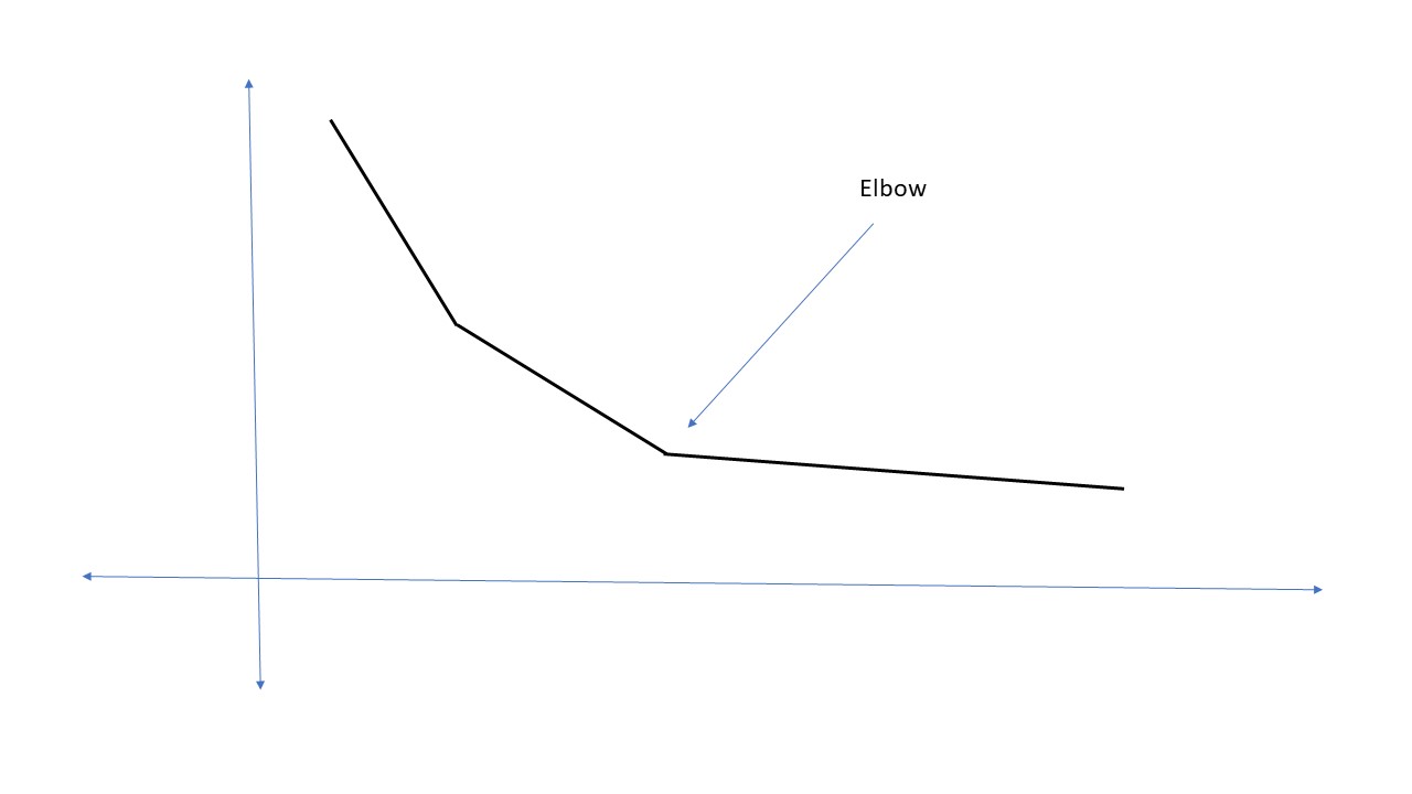
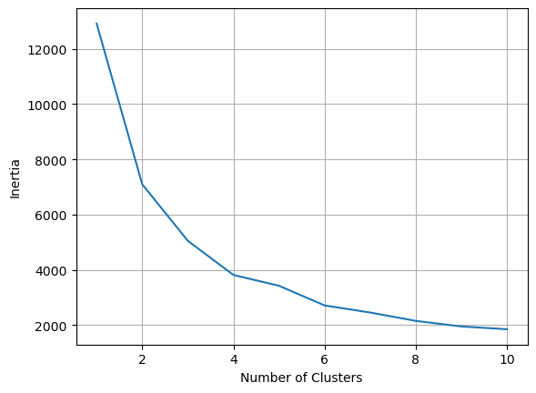
Elbow Rule:

Elbow Point: The point on the inertia curve where the rate of decrease slows significantly, indicating the optimal number of clusters.

Iris data#

from sklearn.datasets import load_iris
X, y = load_iris(return_X_y=True)
f_names = load_iris().feature_names

from sklearn.model_selection import train_test_split
X_train, X_test, y_train, y_test = train_test_split(X, y, random_state=42)

from sklearn.preprocessing import MinMaxScaler
scaler = MinMaxScaler()

# scale the iris data
X_train_scaled = scaler.fit_transform(X_train)
X_test_scaled  = scaler.transform(X_test)

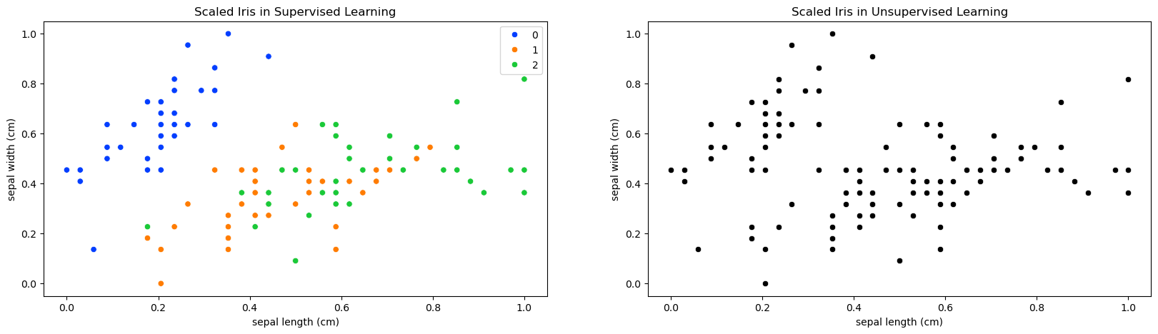
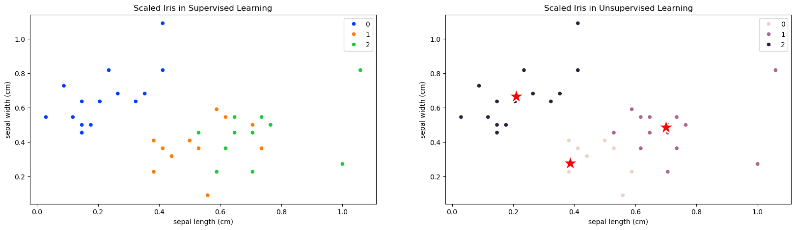
# Iris in Supervised and Unsupervised Learning
import matplotlib.pyplot as plt
import seaborn as sns
plt.figure(figsize=(20,5))
plt.subplot(1,2,1)
plt.title('Scaled Iris in Supervised Learning')
sns.scatterplot( x=X_train_scaled[:,0], y=X_train_scaled[:,1], hue=y_train, palette='bright' )
plt.xlabel(f_names[0])
plt.ylabel(f_names[1])
plt.subplot(1,2,2)
# Iris in Unsupervised Learning
plt.title('Scaled Iris in Unsupervised Learning')
sns.scatterplot( x=X_train_scaled[:,0], y=X_train_scaled[:,1], color='black')
plt.xlabel(f_names[0])
plt.ylabel(f_names[1]);

_images/42431d2fdce97ab0ec58f90fffc10d3cc24ac7ed21a61eb0642441d1f8b09ad1.png

from sklearn.cluster import KMeans
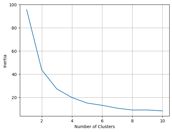
# inertia graph
l_inertia = []
for i in range(1,11):
    kmeans = KMeans(n_clusters = i, n_init='auto')
    kmeans.fit(X_train[:,:2])
    l_inertia.append(kmeans.inertia_)
plt.plot( range(1,11), l_inertia )
plt.xlabel('Number of Clusters')
plt.ylabel('Inertia')
plt.grid();

_images/5f8edeab1ceb182b1afc7bbca521983e3538f39730ab931c963f190a4427c9a6.png

# build the clustering model with 3 clusters
kmeans = KMeans(n_clusters=3, n_init='auto')
kmeans.fit(X_train_scaled[:,:2])

KMeans(n_clusters=3, n_init='auto')

In a Jupyter environment, please rerun this cell to show the HTML representation or trust the notebook.
On GitHub, the HTML representation is unable to render, please try loading this page with nbviewer.org.

kmeans.labels_[:5]

array([2, 2, 0, 1, 1], dtype=int32)

kmeans.cluster_centers_.shape

(3, 2)

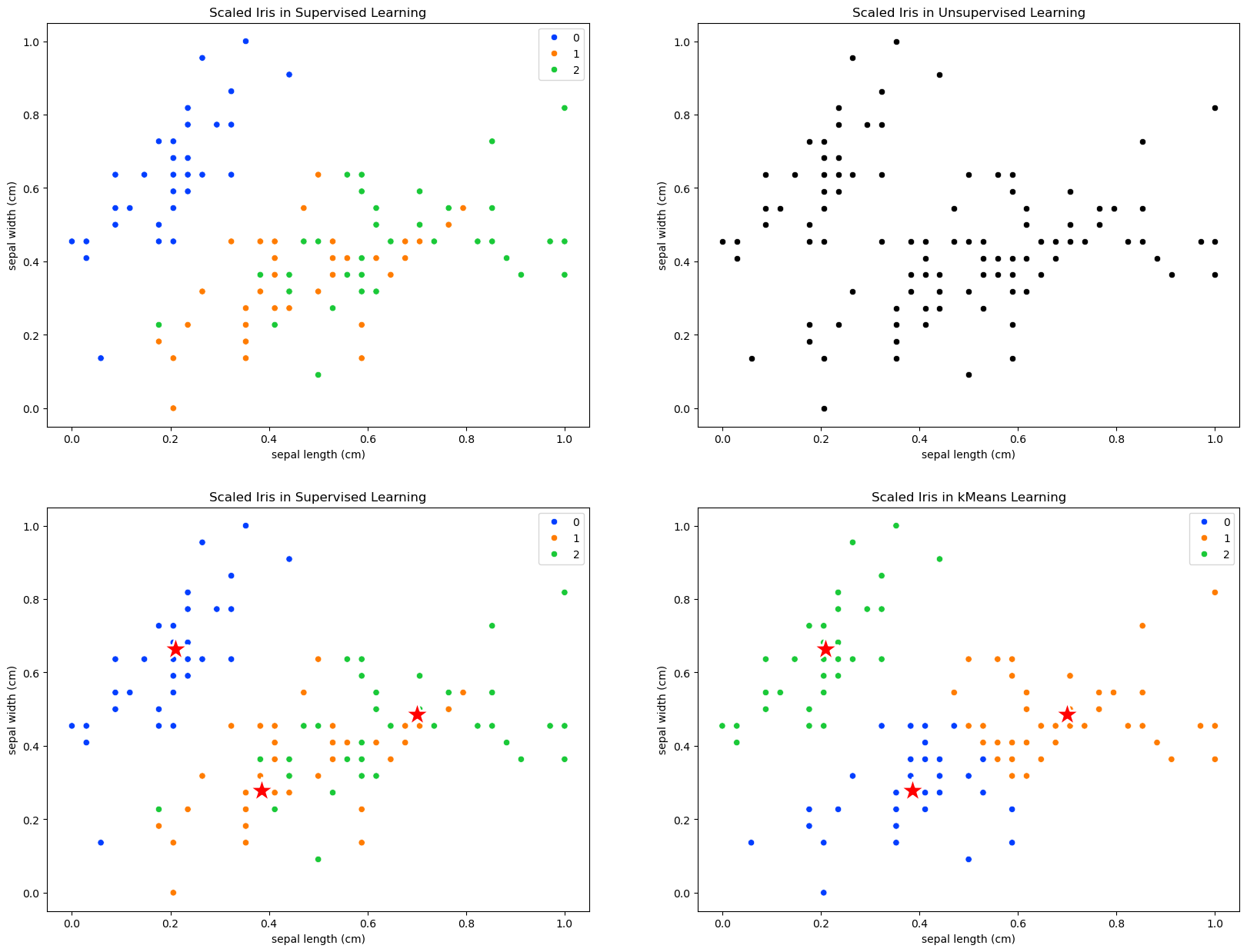
# Iris in Supervised and Unsupervised Learning
plt.figure(figsize=(20,15))
plt.subplot(2,2,1)
plt.title('Scaled Iris in Supervised Learning')
sns.scatterplot( x=X_train_scaled[:,0], y=X_train_scaled[:,1], hue=y_train, palette='bright' )
plt.xlabel(f_names[0])
plt.ylabel(f_names[1])
plt.subplot(2,2,2)
# Iris in Unsupervised Learning
plt.title('Scaled Iris in Unsupervised Learning')
sns.scatterplot( x=X_train_scaled[:,0], y=X_train_scaled[:,1], color='black')
plt.xlabel(f_names[0])
plt.ylabel(f_names[1])
plt.subplot(2,2,3)
# Iris in kMeans Learning
plt.title('Scaled Iris in Supervised Learning')
sns.scatterplot( x=X_train_scaled[:,0], y=X_train_scaled[:,1], hue=y_train, palette='bright' )
sns.scatterplot( x = kmeans.cluster_centers_[:,0], y  = kmeans.cluster_centers_[:,1], color = 'r', marker = '*', s=600 );
plt.xlabel(f_names[0])
plt.ylabel(f_names[1])
plt.subplot(2,2,4)
# Iris in kMeans Learning
plt.title('Scaled Iris in kMeans Learning')
sns.scatterplot( x=X_train_scaled[:,0], y=X_train_scaled[:,1], hue=kmeans.labels_ ,palette='bright')
sns.scatterplot( x = kmeans.cluster_centers_[:,0], y  = kmeans.cluster_centers_[:,1], color = 'r', marker = '*', s=600 );
plt.xlabel(f_names[0])
plt.ylabel(f_names[1])
plt.tight_layout;

_images/8e0c3d2ca4e2ae5d012d157c345837fed75739fa1605444c5e403c8081db95c1.png

# y_train
y_train[:10]

array([0, 0, 2, 1, 1, 0, 0, 1, 2, 2])

# labels
kmeans.labels_[:10]

array([2, 2, 0, 1, 1, 2, 2, 0, 1, 1], dtype=int32)

# Test Set
plt.figure(figsize=(20,5))
plt.subplot(1,2,1)
plt.title('Scaled Iris in Supervised Learning')
sns.scatterplot( x=X_test_scaled[:,0], y=X_test_scaled[:,1], hue=y_test, palette='bright' )
plt.xlabel(f_names[0])
plt.ylabel(f_names[1])
plt.subplot(1,2,2)
# Iris in Unsupervised Learning
plt.title('Scaled Iris in Unsupervised Learning')
sns.scatterplot( x=X_test_scaled[:,0], y=X_test_scaled[:,1], hue=kmeans.predict(X_test_scaled[:,:2]), color='black')
sns.scatterplot( x = kmeans.cluster_centers_[:,0], y  = kmeans.cluster_centers_[:,1], color = 'r', marker = '*', s=600 );
plt.xlabel(f_names[0])
plt.ylabel(f_names[1]);

_images/d807345840ac2bfaeb22939e1c0e6f5dd3da84ab2c235e53dafc79ec07892f07.png

Cancer Dataset#

from sklearn.datasets import load_breast_cancer
X, y = load_breast_cancer(return_X_y=True)
f_names = load_breast_cancer().feature_names

from sklearn.model_selection import train_test_split
X_train, X_test, y_train, y_test = train_test_split(X, y, random_state=42)

from sklearn.preprocessing import MinMaxScaler
scaler = MinMaxScaler()

# scale the iris data
X_train_scaled = scaler.fit_transform(X_train)
X_test_scaled  = scaler.transform(X_test)

# inertia graph
l_inertia = []
for i in range(1,11):
    kmeans = KMeans(n_clusters = i, n_init='auto')
    kmeans.fit(X_train[:,:2])
    l_inertia.append(kmeans.inertia_)
plt.plot( range(1,11), l_inertia )
plt.xlabel('Number of Clusters')
plt.ylabel('Inertia')
plt.grid();

_images/9425a3d05090ae24c10e33e5cb3eefd2dbd9cd7d5d5f61d120c1f7e70a6a1275.png

# n_clusters=2
kmeans = KMeans(n_clusters=2, n_init='auto')
kmeans.fit(X_train_scaled[:,:2])

KMeans(n_clusters=2, n_init='auto')

In a Jupyter environment, please rerun this cell to show the HTML representation or trust the notebook.
On GitHub, the HTML representation is unable to render, please try loading this page with nbviewer.org.

kmeans.labels_[:5]

array([0, 0, 0, 1, 1], dtype=int32)

kmeans.cluster_centers_.shape

(2, 2)

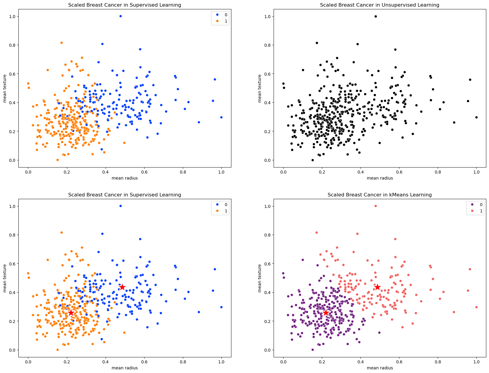
# Breast Cancer Data in Supervised and Unsupervised Learning
plt.figure(figsize=(20,15))
plt.subplot(2,2,1)
plt.title('Scaled Breast Cancer in Supervised Learning')
sns.scatterplot( x=X_train_scaled[:,0], y=X_train_scaled[:,1], hue=y_train, palette='bright' )
plt.xlabel(f_names[0])
plt.ylabel(f_names[1])
plt.subplot(2,2,2)
# bc in Unsupervised Learning
plt.title('Scaled Breast Cancer in Unsupervised Learning')
sns.scatterplot( x=X_train_scaled[:,0], y=X_train_scaled[:,1], color='black')
plt.xlabel(f_names[0])
plt.ylabel(f_names[1])
plt.subplot(2,2,3)
# bc in kMeans Learning
plt.title('Scaled Breast Cancer in Supervised Learning')
sns.scatterplot( x=X_train_scaled[:,0], y=X_train_scaled[:,1], hue=y_train, palette='bright' )
sns.scatterplot( x = kmeans.cluster_centers_[:,0], y  = kmeans.cluster_centers_[:,1], color = 'r', marker = '*', s=600 );
plt.xlabel(f_names[0])
plt.ylabel(f_names[1])
plt.subplot(2,2,4)
# bc in kMeans Learning
plt.title('Scaled Breast Cancer in kMeans Learning')
sns.scatterplot( x=X_train_scaled[:,0], y=X_train_scaled[:,1], hue=kmeans.labels_ ,palette='magma')
sns.scatterplot( x = kmeans.cluster_centers_[:,0], y  = kmeans.cluster_centers_[:,1], color = 'r', marker = '*', s=600 );
plt.xlabel(f_names[0])
plt.ylabel(f_names[1])
plt.tight_layout;

_images/d7fdb6edf19cdc5f567bc6e971350106145f6834b4cccc0cc95a059fef9fe639.png

# first 10 y_train
y_train[:10]

array([1, 0, 1, 0, 0, 0, 1, 0, 1, 1])

# first 10 labels
kmeans.labels_[:10]

array([0, 0, 0, 1, 1, 1, 0, 1, 0, 0], dtype=int32)

# success ratio
1-sum(y_train == kmeans.labels_)/len(X_train_scaled)

0.8849765258215962

# kMeans with whole features
kmeans.fit(X_train_scaled)
sum(y_train == kmeans.labels_)/len(X_train_scaled)

0.9131455399061033

# kMeans with whole features on test data
sum(y_test == kmeans.predict(X_test_scaled))/len(X_test_scaled)

0.9440559440559441

K-means

Contents

K-means#

Iris data#

Cancer Dataset#