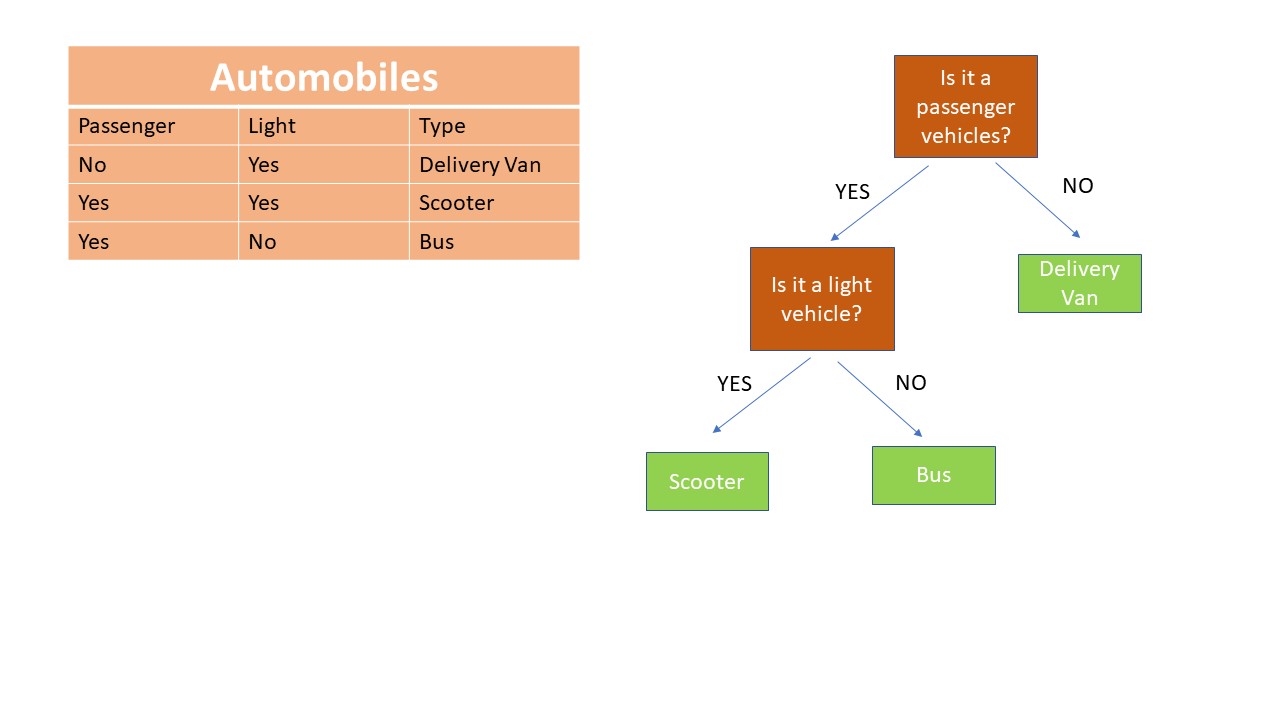
Decision Tree#

It consists of a ordered hierarchy of if/else questions.
Decision trees can be used for both classification and regression tasks.
The model predicts the value of an output (target variable) by answering these if/else questions.
Each question splits the samples into two subsamples.
The goal is to find the smallest tree that fits the data. In other words, asking as few questions as possible.
If a feature is a continuous variable, the questions involve determining whether the feature value is less than or equal to a specific number, known as the threshold.
The decision tree algorithm determines the questions based on the feature and the threshold when dealing with continuous variables.
The initial node is referred to as the root, while a terminal node is called a leaf.
Decision Tree Classifier#
from sklearn.datasets import load_breast_cancer
X, y = load_breast_cancer(return_X_y=True)
from sklearn.model_selection import train_test_split
X_train, X_test, y_train, y_test = train_test_split(X, y, random_state=0)
from sklearn.tree import DecisionTreeClassifier
dt = DecisionTreeClassifier(random_state=0)
dt.fit(X_train, y_train)
DecisionTreeClassifier(random_state=0)In a Jupyter environment, please rerun this cell to show the HTML representation or trust the notebook.
On GitHub, the HTML representation is unable to render, please try loading this page with nbviewer.org.
DecisionTreeClassifier(random_state=0)
dt.score(X_train, y_train)
1.0
dt.score(X_test, y_test)
0.8811188811188811
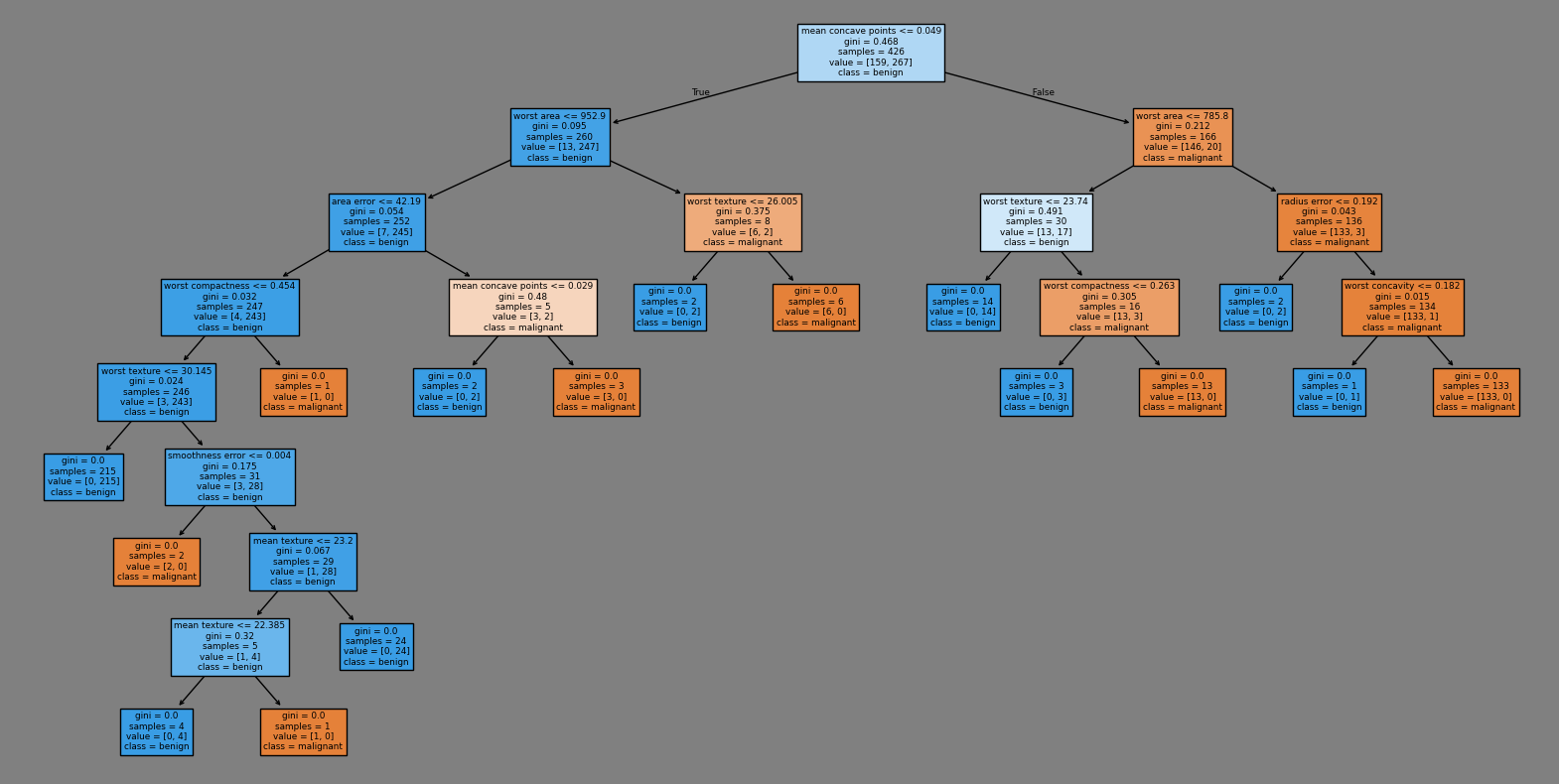
# sketch the tree
from sklearn import tree
import matplotlib.pyplot as plt
fig, ax = plt.subplots(figsize=(20, 10), facecolor='gray')

tree.plot_tree(dt, filled=True, class_names=load_breast_cancer().target_names, feature_names=load_breast_cancer().feature_names, ax=ax);
max_depth#
dt = DecisionTreeClassifier(max_depth=2, random_state=0)
dt.fit(X_train, y_train)
fig, ax = plt.subplots(figsize=(20,7), facecolor='gray')
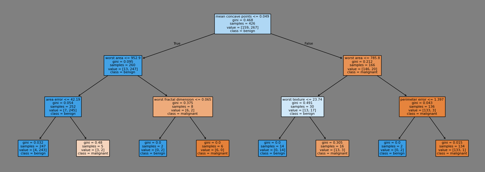
tree.plot_tree(dt, filled=True, class_names=load_breast_cancer().target_names, feature_names=load_breast_cancer().feature_names, ax=ax);
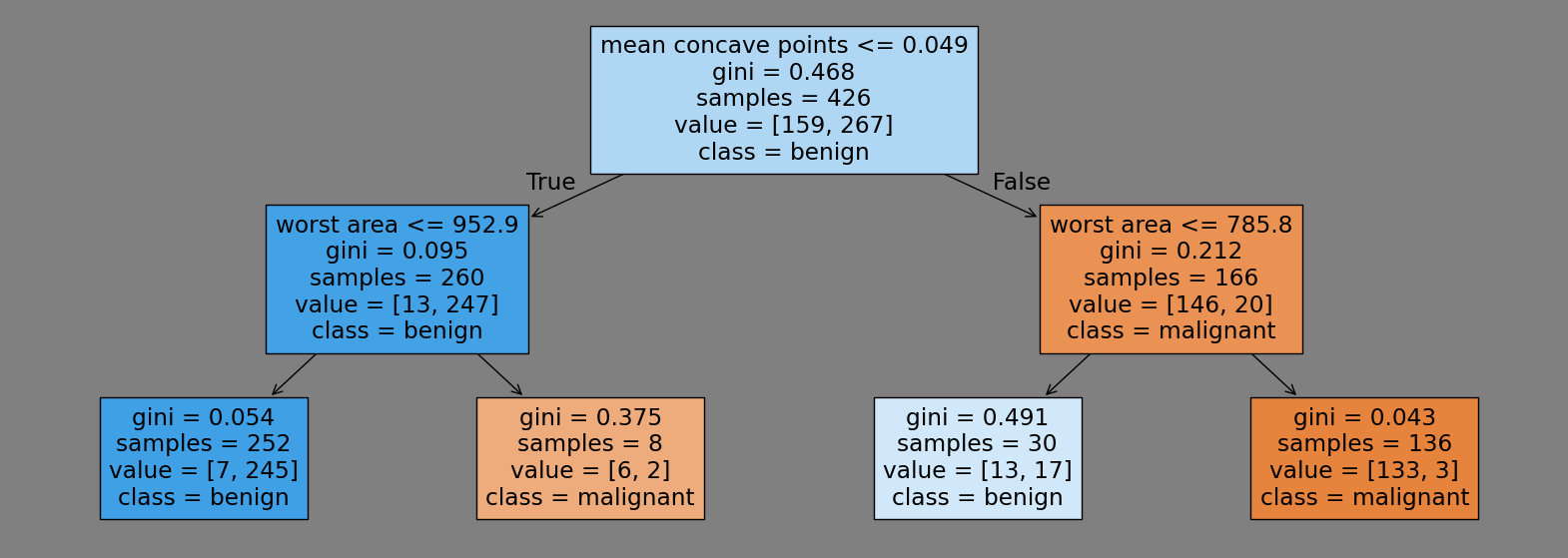
Gini Impurity#
In classification tasks, Gini Impurity is used to select the questions in the decision tree.
The Gini Impurity \(G\) is calculated using the formula: \(G = 1- \sum p_i^2\), where \(p_i\) represents the probability of each class in the node.
The question that minimizes the Gini Impurity is chosen.
For the node in the bottom left corner above, the Gini Impurity is calculated as follows and the output is 0.054:
round(1-(7/252)**2-(245/252)**2, 3)
In regression tasks, the mean squared error (MSE) is used instead of Gini Impurity.
dt = DecisionTreeClassifier(max_depth=3, random_state=0)
dt.fit(X_train, y_train)

fig, ax = plt.subplots(figsize=(20,7), facecolor='gray')

tree.plot_tree(dt, filled=True, class_names=load_breast_cancer().target_names, feature_names=load_breast_cancer().feature_names, ax=ax);
for md in [2, 4, 6, 8, 10]:
    dt = DecisionTreeClassifier(max_depth=md, random_state=0)
    dt.fit(X_train, y_train)
    print(f'Max Depth: {md} --- Training Score: {dt.score(X_train, y_train):.2f} --- Test Score: {dt.score(X_test, y_test):.2f}')
Max Depth: 2 --- Training Score: 0.94 --- Test Score: 0.94
Max Depth: 4 --- Training Score: 0.99 --- Test Score: 0.90
Max Depth: 6 --- Training Score: 1.00 --- Test Score: 0.92
Max Depth: 8 --- Training Score: 1.00 --- Test Score: 0.88
Max Depth: 10 --- Training Score: 1.00 --- Test Score: 0.88
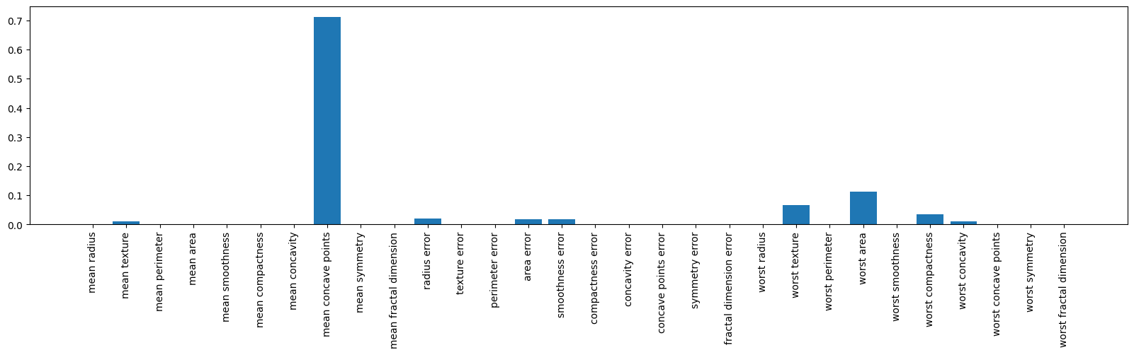
Feature Importances#
The feature_importances_ attribute returns the significance of each feature in building the model using the Decision Tree algorithm.
The sum of the importances for all features equals 1.
dt.feature_importances_
array([0.        , 0.0096886 , 0.        , 0.        , 0.        ,
       0.        , 0.        , 0.71160121, 0.        , 0.        ,
       0.01948008, 0.        , 0.        , 0.01676117, 0.017502  ,
       0.        , 0.        , 0.        , 0.        , 0.        ,
       0.        , 0.06706044, 0.        , 0.11373562, 0.        ,
       0.03421113, 0.00995974, 0.        , 0.        , 0.        ])
plt.figure(figsize=(20,4))
plt.bar(load_breast_cancer().feature_names, dt.feature_importances_)
plt.xticks(rotation=90);
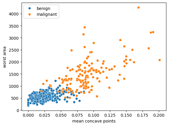
2-feature Case#
feature_importances_list = list(load_breast_cancer().feature_names)
target_names = load_breast_cancer().target_names

index_mcp = feature_importances_list.index('mean concave points')
index_wa  = feature_importances_list.index('worst area')
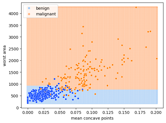
import seaborn as sns
sns.scatterplot(x=X_train[:,index_mcp], y=X_train[:,index_wa], hue=[target_names[i] for i in y_train])
plt.xlabel('mean concave points')
plt.ylabel('worst area');
dt = DecisionTreeClassifier(random_state=0, max_depth=2)
dt.fit(X_train[:,[index_mcp, index_wa]], y_train)
DecisionTreeClassifier(max_depth=2, random_state=0)In a Jupyter environment, please rerun this cell to show the HTML representation or trust the notebook.
On GitHub, the HTML representation is unable to render, please try loading this page with nbviewer.org.
DecisionTreeClassifier(max_depth=2, random_state=0)
fig, ax = plt.subplots(figsize=(20,7), facecolor='gray')

tree.plot_tree(dt, filled=True, class_names=target_names, feature_names=['mean concave points', 'worst area'], ax=ax);
Decision Boundary#
import numpy as np
N = 100
x1_values = np.linspace( min(X_train[:,index_mcp]), max(X_train[:,index_mcp]), N )
x2_values = np.linspace( min(X_train[:,index_wa]), max(X_train[:,index_wa]), N )

x_values = [(x1,x2) for x1 in x1_values for x2 in x2_values]
x1_values = [i[0] for i in x_values]
x2_values = [i[1] for i in x_values]

y_pred = dt.predict(x_values)
sns.scatterplot(x=x1_values, y=x2_values, hue=[target_names[i] for i in y_pred], palette='bright')
plt.xlabel('mean concave points')
plt.ylabel('worst area');
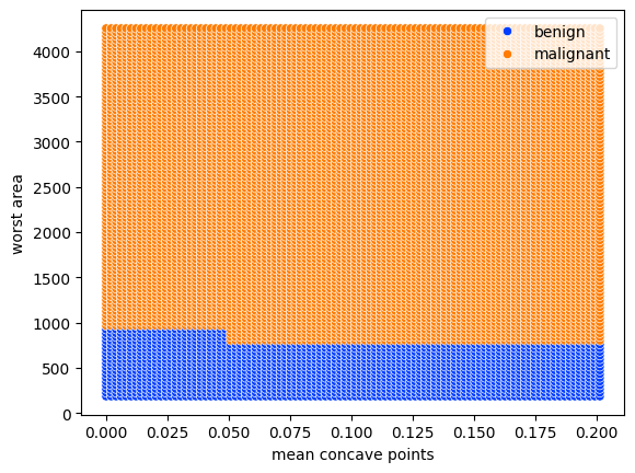
sns.scatterplot(x=x1_values, y=x2_values, hue=[target_names[i] for i in y_pred], palette='pastel')
plt.xlabel('mean concave points')
plt.ylabel('worst area')

sns.scatterplot(x=X_train[:,index_mcp], y=X_train[:,index_wa],
                hue=[target_names[i] for i in y_train], s=20,
                palette='bright', legend=False);
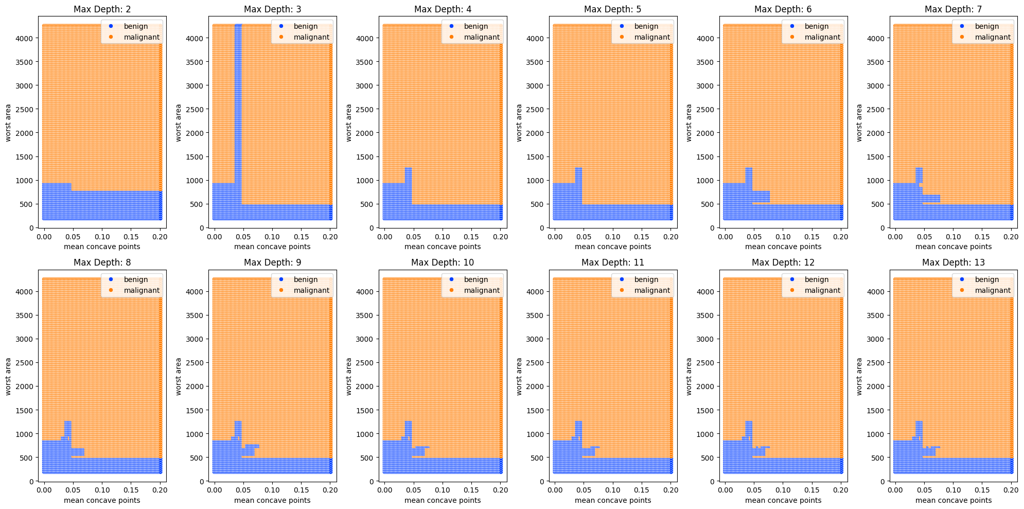
plt.figure(figsize=(20,10))
for md in range(2,14):
    plt.subplot(2,6,md-1)
    dt = DecisionTreeClassifier(random_state=0, max_depth=md)
    dt.fit(X_train[:,[index_mcp, index_wa]], y_train)
    y_pred = dt.predict(x_values)
    sns.scatterplot(x=x1_values, y=x2_values, hue=[target_names[i] for i in y_pred], palette='bright')
    plt.xlabel('mean concave points')
    plt.ylabel('worst area')
    plt.title(f'Max Depth: {md}')
    plt.tight_layout()
Decision Tree Regressor#
from sklearn.datasets import fetch_california_housing
X, y = fetch_california_housing(return_X_y=True)
from sklearn.model_selection import train_test_split
X_train, X_test, y_train, y_test = train_test_split(X, y, random_state=0)
from sklearn.tree import DecisionTreeRegressor
dt = DecisionTreeRegressor(random_state=0)
dt.fit(X_train, y_train)
DecisionTreeRegressor(random_state=0)In a Jupyter environment, please rerun this cell to show the HTML representation or trust the notebook.
On GitHub, the HTML representation is unable to render, please try loading this page with nbviewer.org.
DecisionTreeRegressor(random_state=0)
dt.score(X_train, y_train)
1.0
dt.score(X_test, y_test)
0.5859590482097172
max_depth#
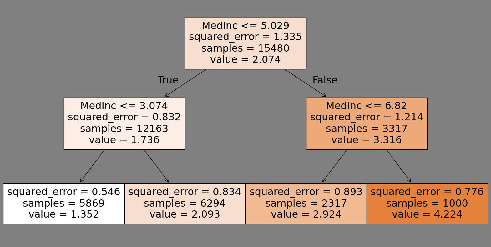
dt = DecisionTreeRegressor(max_depth=2, random_state=0)
dt.fit(X_train, y_train)

fig, ax = plt.subplots(figsize=(20,10), facecolor='gray')
tree.plot_tree(dt, filled=True, feature_names=fetch_california_housing().feature_names, ax=ax);
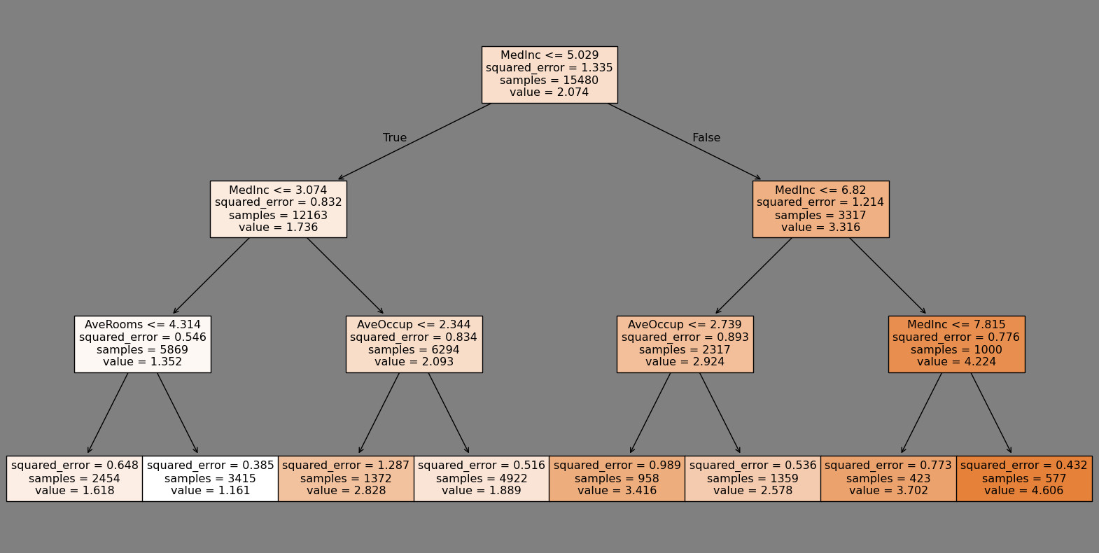
dt = DecisionTreeRegressor(max_depth=3, random_state=0)
dt.fit(X_train, y_train)

fig, ax = plt.subplots(figsize=(20,10), facecolor='gray')
tree.plot_tree(dt, filled=True, feature_names=fetch_california_housing().feature_names, ax=ax);
for md in [2, 4, 6, 7, 8, 10, 12, 14, 16, 18, 20]:
    dt = DecisionTreeRegressor(max_depth=md, random_state=0)
    dt.fit(X_train, y_train)
    print(f'Max Depth: {md} --- Training Score: {dt.score(X_train, y_train):.2f} --- Test Score: {dt.score(X_test, y_test):.2f}')
Max Depth: 2 --- Training Score: 0.45 --- Test Score: 0.43
Max Depth: 4 --- Training Score: 0.59 --- Test Score: 0.55
Max Depth: 6 --- Training Score: 0.68 --- Test Score: 0.62
Max Depth: 7 --- Training Score: 0.71 --- Test Score: 0.65
Max Depth: 8 --- Training Score: 0.76 --- Test Score: 0.67
Max Depth: 10 --- Training Score: 0.84 --- Test Score: 0.68
Max Depth: 12 --- Training Score: 0.90 --- Test Score: 0.65
Max Depth: 14 --- Training Score: 0.95 --- Test Score: 0.62
Max Depth: 16 --- Training Score: 0.98 --- Test Score: 0.60
Max Depth: 18 --- Training Score: 0.99 --- Test Score: 0.59
Max Depth: 20 --- Training Score: 1.00 --- Test Score: 0.59
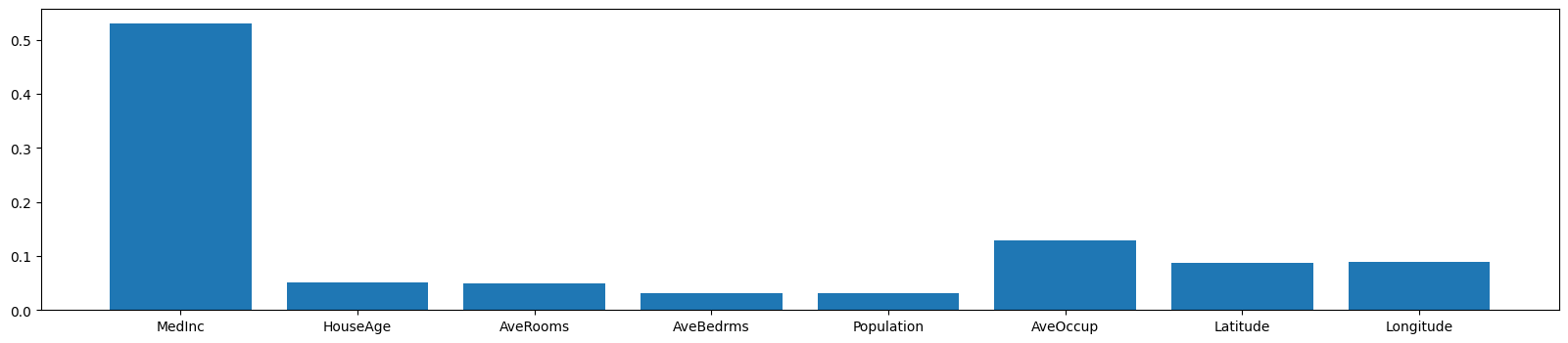
Feature Importances#
dt.feature_importances_
array([0.53035558, 0.05191171, 0.04940284, 0.03064305, 0.03178456,
       0.12956303, 0.08688653, 0.08945269])
plt.figure(figsize=(20,4))
plt.bar(fetch_california_housing().feature_names, dt.feature_importances_);