Numpy Arrays

Motivation

Let’s attempt to multiply each element of a list by 10.

• The * operator repeats the list elements.

• If we use the * operator on a list, instead of multiplying each element by 10, it replicates the initial list 10 times, as shown in the following code:

list1 = [1,2,3]
print(list1*10)

[1, 2, 3, 1, 2, 3, 1, 2, 3, 1, 2, 3, 1, 2, 3, 1, 2, 3, 1, 2, 3, 1, 2, 3, 1, 2, 3, 1, 2, 3]

• We can multiply each element of a list using list comprehensions.

new_list = [i*10 for i in list1]
print(new_list)

[10, 20, 30]

• However, it’s quite common to multiply each element of a sequence by a fixed number, and there should be a more efficient way to accomplish this.

• NumPy arrays interpret the * operator as multiplication, not repetition.

import numpy as np
array1 = np.array([1,2,3])
print(array1)

[1 2 3]

print(array1*10)

[10 20 30]

There’s a similar situation with the + operator.

• For lists, + concatenates elements, whereas for NumPy arrays, it performs componentwise addition.

list1 = [1,2,3]
list2 = [4,5,6]
print(list1+list2)

[1, 2, 3, 4, 5, 6]

array1 = np.array([1,2,3])
array2 = np.array([4,5,6])
print(array1+array2)

[5 7 9]

Numpy

Numpy is the foundational package for scientific computing in Python.

• Numpy’s primary data structure is arrays.

  • Arrays are known for their speed and versatility.

  • They enable vectorized operations.

  • Indexing facilitates accessing values within an array.

• NumPy offers a comprehensive collection of mathematical tools for various computations, encompassing:

  • Matrix operations

  • Generation of random numbers

  • Mathematical and statistical functions

• NumPy methods can be used for importing and manipulating images.

• NumPy is the foundation for powerful machine learning libraries like scikit-learn and SciPy.

• It’s customary to import the numpy package under the alias np for brevity and clarity in code.

import numpy as np

Numpy Arrays

A NumPy array, also known as ndarray is a multidimensional array.

• You can perform mathematical and statistical operations on arrays.

• Manipulations such as reshaping, sorting, stacking, transposing, and shuffling arrays are possible.

The np.array() method is used to create an array. The following code generates a 2 by 3 matrix.

myarray = np.array([ [1,2,3], [4,5,6]])
print(myarray)

[[1 2 3]
 [4 5 6]]

The type of a NumPy array is ndarray.

print(type(myarray))

<class 'numpy.ndarray'>

The following is an example of an array with string values:

np.array(['a', 'b', 'c', 'd', 'e'])

array(['a', 'b', 'c', 'd', 'e'], dtype='<U1')

Dimensions

The dimension of a numpy array is the number of axes along which the array extends.

• Examples:

  • Vector: A one-dimensional array. It has only one axis.

  • Matrix (Grid): A two-dimensional array. It has two axes.

• The dimension of an array indicates the number of indices required to specify an element within the array.

• The dimension of an array can be determined using the ndim attribute.

0-dimension

Its elements consist of scalars like single numbers.

np.array(5)

array(5)

myarray0 = np.array(5)
print(myarray0.ndim)

0

1-dimension

Its elements consist of 0-dimensional arrays.

• 1,2,3,4 are 0 dimensional.

myarray1 = np.array([1,2,3,4])
print(myarray1.ndim)

1

2-dimension

Its elements consist of 1-dimensional arrays.

• [1,2] annd [3,4] are 1-dimensional.

myarray2 = np.array([[1,2],[3,4]])
print('Dimension:', myarray2.ndim)
print('='*15)
print( myarray2)

Dimension: 2
===============
[[1 2]
 [3 4]]

3-dimension

Its elements consist of 2-dimensional arrays.

• [[1,2],[3,4]], [[5,6],[7,8]], [[9,10],[11,12]] are 2-dimensional.

myarray3 = np.array( [[[1,2],[3,4]],[[5,6],[7,8]], [[9,10],[11,12]]] )
print('Dimension:', myarray3.ndim)
print('='*15)
print( myarray3)

Dimension: 3
===============
[[[ 1  2]
  [ 3  4]]

 [[ 5  6]
  [ 7  8]]

 [[ 9 10]
  [11 12]]]

Shape

The shape of a numpy array is the number of elements in each dimension.

• Since the dimension of the following array is 3, its shape consists of three numbers.

myarray = np.array( [[[1,1,1,1],[2,2,2,2], [3,3,3,3]], [[4,4,4,4],[5,5,5,5], [6,6,6,6]]] )
print('Dimension:', myarray3.ndim)
print('-'*15)
print( myarray)

Dimension: 3
---------------
[[[1 1 1 1]
  [2 2 2 2]
  [3 3 3 3]]

 [[4 4 4 4]
  [5 5 5 5]
  [6 6 6 6]]]

• In the first dimension: There are two elements: [[1,1,1,1],[2,2,2,2], [3,3,3,3]] and [[4,4,4,4],[5,5,5,5], [6,6,6,6]]].

• In the second dimension each element has 3 elements.

  • [[1,1,1,1],[2,2,2,2], [3,3,3,3]] has 3 elements [1,1,1,1],[2,2,2,2], and [3,3,3,3].

  • [[4,4,4,4],[5,5,5,5], [6,6,6,6]] has 3 elements [4,4,4,4],[5,5,5,5], and [6,6,6,6].

• In the third dimension there are 4 elements of each element.

  • [1,1,1,1], [2,2,2,2],…., [6,6,6,6] are all have four elements.

print('Shape    :', myarray.shape)

Shape    : (2, 3, 4)

Example

myarray = np.array( [[[1],[2], [3]]] )
print('Dimension:', myarray.ndim)
print('Shape    :', myarray.shape)
print('-'*15)
print( myarray)

Dimension: 3
Shape    : (1, 3, 1)
---------------
[[[1]
  [2]
  [3]]]

• In the first dimension: There is only element: [[1],[2], [3]].

• In the second dimension: [[1],[2], [3]] has 3 elements.

• In the third dimension: there is 1 element of each element.

  • [1],[2], [3] are all have one element.

Example

myarray = np.array( [[[[1]]]] )
print('Dimension:', myarray.ndim)
print('Shape    :', myarray.shape)
print('-'*15)
print( myarray)

Dimension: 4
Shape    : (1, 1, 1, 1)
---------------
[[[[1]]]]

• In the first dimension: There is only elements: [[[1]]].

• In the second dimension: [[[1]]] has 1 element: [[1]]

• In the third dimension: [[1]] has 1 element: [1].

• In the fourth dimension: [1] has 1 element: 1.

Example

myarray = np.array( [1,2,3])
print('Dimension:', myarray.ndim)
print('Shape    :', myarray.shape)
print('-'*15)
print( myarray)

Dimension: 1
Shape    : (3,)
---------------
[1 2 3]

There is only one dimension and there are 3 elements in this dimension.

Size

• The total number of elements.

myarray = np.array( [[[1],[2], [3]]] )
print('Dimension:', myarray.ndim)
print('Shape    :', myarray.shape)
print('Size     :', myarray.size)

print('-'*15)
print( myarray)

Dimension: 3
Shape    : (1, 3, 1)
Size     : 3
---------------
[[[1]
  [2]
  [3]]]

myarray = np.array( [[[1,1,1,1],[2,2,2,2], [3,3,3,3]], [[4,4,4,4],[5,5,5,5], [6,6,6,6]]] )
print('Dimension:', myarray.ndim)
print('Shape    :', myarray.shape)
print('Size     :', myarray.size)

print('-'*15)
print( myarray)

Dimension: 3
Shape    : (2, 3, 4)
Size     : 24
---------------
[[[1 1 1 1]
  [2 2 2 2]
  [3 3 3 3]]

 [[4 4 4 4]
  [5 5 5 5]
  [6 6 6 6]]]

Indexing

Indexing of ndarrays involves square brackets, just like with lists.

• When using indexing, you can consider the ndarray as lists of lists.

myarray = np.array( [[3, 5, 7], [2, 9, 8]] )
print(myarray)

[[3 5 7]
 [2 9 8]]

# index 0 element of [[3, 5, 7], [2, 9, 8]] 
myarray[0]

array([3, 5, 7])

# index 2 element of [3, 5, 7]
myarray[0][2]

7

Instead of using double square brackets, the notation can also be simplified as follows:

• [0][2] is equivalent to [0, 2].

# row index: 0, column index:2
myarray[0,2]

7

Slicing

The colon (:) is used for slicing, just like with lists.

myarray

array([[3, 5, 7],
       [2, 9, 8]])

# all rows, columns starting from index 1
myarray[:,1:]

array([[5, 7],
       [9, 8]])

Mutable

NumPy arrays are mutable, meaning their elements can be modified.

In the following code, we demonstrate how to change specific values in a NumPy array:

myarray

array([[3, 5, 7],
       [2, 9, 8]])

We will change the value at index [1, 2] in the NumPy array. Here’s how it can be done:

• The row at index 1 is [9, 6, 7].

• The element at index 2 in this row is 7.

• We will replace this value with 99.

myarray[1,2] = 99
myarray

array([[ 3,  5,  7],
       [ 2,  9, 99]])

Mixed Datatypes

A NumPy array can store mixed data types, but it will convert all elements to a single data type that can accommodate all the types present in the array. For example:

• If integers and floats are mixed, the array will store them as floats.

• If numbers and strings are mixed, the array will store all elements as strings.

In the example below, all values are stored as strings.

array = np.array([1,2,'a'])
array

array(['1', '2', 'a'], dtype='<U21')

Vectorized Operations

The advantage of using vectorized operations in NumPy is that they make computations faster and easier by applying operations directly to entire arrays, without needing to loop through each element one by one.

We will use the following arrays to perform component-wise operations, where each operation is applied individually to corresponding elements of the arrays:

array1 = np.array( [3, 5, 7] )
array2 = np.array( [2, 9, 8] )

Addition

\([3, 5, 7]+[2, 9, 8]=[3+2, 5+9, 7+8]=[ 5, 14, 15]\)

array1 + array2 

array([ 5, 14, 15])

Multiplication

\([3, 5, 7]*[2, 9, 8]=[3*2, 5*9, 7*8]=[ 6, 45, 56]\)

array1 * array2 

array([ 6, 45, 56])

Exponent

\([3, 5, 7]^2=[3^2, 5^9, 7^8]=[9, 25, 49]\)

array1**2

array([ 9, 25, 49])

Comparison Operators

\([3, 5, 7]>6=[3>6, 5>6, 7>6]=[ False, False, True]\)

array1 > 6

array([False, False,  True])

def sq(x):
    return x**2

sq(array1)

array([ 9, 25, 49])

Array Methods

reshape()

• The reshape() method generates a new array with the specified shape.

array1 = np.array([1,2,3,4,5,6])
print('Dimension:', array1.ndim)
print('Shape    :', array1.shape)

Dimension: 1
Shape    : (6,)

array2 = array1.reshape(2,3)
print('='*15)
print('New Array')
print('Dimension:', array2.ndim)
print('Shape    :', array2.shape)
print('='*15)
print(array2)

===============
New Array
Dimension: 2
Shape    : (2, 3)
===============
[[1 2 3]
 [4 5 6]]

sum()

• sum(): sum of all elements

• sum(0): sum for each column (in 2 dim)

• sum(1): sum for each row (in 2 dim)

myarray = np.array( [[1,2,3],[4,5,6]] )
print(myarray)

[[1 2 3]
 [4 5 6]]

# 1+2+3+4+5+6
print(myarray.sum())

21

# 1+4=5
# 2+5=7
# 3+6=9
print(myarray.sum(0))

[5 7 9]

# 1+2+3=6
# 4+5+6=15
print(myarray.sum(1))

[ 6 15]

min()

• min(): minimum of all elements

• min(0): minimum for each column (in 2 dim)

• min(1): minimum for each row (in 2 dim)

myarray = np.array( [ [3,5,7], [2,9,8] ] )
print(myarray)

[[3 5 7]
 [2 9 8]]

# minimum of 3, 5, 7, 2, 9, 8
print(myarray.min())

2

# minimum of 3, 2
# minimum of 5, 9
# minimum of 7, 8

print(myarray.min(0))

[2 5 7]

# minimum of 3, 5, 7
# minimum of 2, 9, 8

print(myarray.min(1))

[3 2]

max()

• max(): maximum of all elements

• max(0): maximum for each column (in 2 dim)

• max(1): maximum for each row (in 2 dim)

myarray = np.array( [ [3,5,7], [2,9,8] ] )
print(myarray)

[[3 5 7]
 [2 9 8]]

# maximum of 3, 5, 7, 2, 9, 8
print(myarray.max())

9

# maximum of 3, 2
# maximum of 5, 9
# maximum of 7, 8

print(myarray.max(0))

[3 9 8]

# maximum of 3, 5, 7
# maximum of 2, 9, 8

print(myarray.max(1))

[7 9]

sort()

The sort() method sorts the values in an array and modifies the original array.

myarray = np.array( [1,9,4,0,2,7,5] )
myarray.sort()
print(myarray)

[0 1 2 4 5 7 9]

# colum-wise sorting
myarray = np.array( [[1,9,4],[2,7,5]] )
myarray.sort(0)
print(myarray)

[[1 7 4]
 [2 9 5]]

# row-wise sorting
myarray = np.array( [[1,9,4],[2,7,5]] )
myarray.sort(1)
print(myarray)

[[1 4 9]
 [2 5 7]]

# default: row-wise
myarray = np.array( [[1,9,4],[2,7,5]])
myarray.sort()
print(myarray)

[[1 4 9]
 [2 5 7]]

argmin()

The argmin() method returns the index of the minimum element.

# minimum element: 3
# index of 3 is 1
myarray = np.array( [5,3,9,6])
print(myarray.argmin())

1

argmax()

The argmax() method returns the index of the maximum element.

# maximum element: 9
# index of 9 is 2
myarray = np.array( [5,3,9,6])
print(myarray.argmax())

2

astype()

The astype() method is used to convert the data type of the elements in a NumPy array to a specified type.

array = np.array([1, 2.34, 7])
array

array([1.  , 2.34, 7.  ])

The following example converts the values of the array into string type using the astype() method.

array.astype('str')

array(['1.0', '2.34', '7.0'], dtype='<U32')

The following example converts the values of the array into integer type using the astype() method.

array.astype('int')

array([1, 2, 7])

Numpy Methods

hstack()

The hstack() method combines arrays column-wise or horizontally.

array1 = np.array([1,2,3])
array2 = np.array([4,5,6])
print(np.hstack([array1, array2]))

[1 2 3 4 5 6]

vstack()

The hstack() method combines arrays row-wise or vertically.

array1 = np.array([1,2,3])
array2 = np.array([4,5,6])
print(np.vstack([array1, array2]))

[[1 2 3]
 [4 5 6]]

linspace()

The linspace() method calculates and returns a specific number of evenly spaced samples within the provided interval, including both the start and stop values.

• You can choose whether or not to include the endpoint of the interval.

The following code generates 20 numbers starting from 2 and ends up at 10.

• The difference between each consecutive number is \((10-2)/(20-1)\)

• 1 is subtracted from 20 because there are 19 intervals between 20 numbers.

# start=10, end=10, number of generated numbers:20
np.linspace(2,10,20) 

array([ 2.        ,  2.42105263,  2.84210526,  3.26315789,  3.68421053,
        4.10526316,  4.52631579,  4.94736842,  5.36842105,  5.78947368,
        6.21052632,  6.63157895,  7.05263158,  7.47368421,  7.89473684,
        8.31578947,  8.73684211,  9.15789474,  9.57894737, 10.        ])

To exclude the endpoint, set the endpoint parameter to False.

np.linspace(2,10,5, endpoint=False)

array([2. , 3.6, 5.2, 6.8, 8.4])

round()

The round() function rounds the elements of an array to the specified number of decimal places. Its syntax is numpy.around(a, decimals=0, out=None).

array = np.array([[1.8945, 3.4216],[5.8253, 6.01632]])
np.round( array, 2)

array([[1.89, 3.42],
       [5.83, 6.02]])

where()

The numpy.where() function selects elements from either x or y based on the given condition.

• If the condition is True, it returns elements from x; otherwise, it returns elements from y.

• Its syntax is numpy.where(condition, x, y).

array = np.array([[5, 0],[1, 3]])
np.where(array>2, 'Large', 'Small')

array([['Large', 'Small'],
       ['Small', 'Large']], dtype='<U5')

select()

The numpy.select() function selects elements in choicelist, depending on condition(s).

• If the condition is True, it returns the corresponding value in the choicelist.

• Its syntax is numpy.select(condlist, choicelist)

array = np.array([[5, 0],[1, 3]])
np.select([True, False], ['a', 'b'])

array('a', dtype='<U3')

dot()

The dot() method returns the dot product of two vectors, which is the sum of their componentwise products.

Example:
\( [1,2,3] \cdot [4,5,6] = 1\cdot 4 + 2\cdot 5+ 3\cdot 6 = 4+10+18=32 \)

array1 = np.array([1,2,3])
array2 = np.array([4,5,6])

print(np.dot(array1,array2))

32

cross()

The cross() method returns the cross product of two vectors.

array1 = np.array([1,2,3])
array2 = np.array([4,5,6])

print(np.cross(array1,array2))

[-3  6 -3]

zeros()

The zeros() method creates an array of the specified size where all elements are initialized to 0.

np.zeros((4,2))

array([[0., 0.],
       [0., 0.],
       [0., 0.],
       [0., 0.]])

ones()

It creates an array of the specified size where all elements are initialized to 1.

np.ones((4,2))

array([[1., 1.],
       [1., 1.],
       [1., 1.],
       [1., 1.]])

Random Module

NumPy’s random module can be used to generate randomly selected values in an array format.

randint()

It generates random integers between the specified low and high values (inclusive for low and exclusive for high) using the format: random.randint(low, high=None, size=None, dtype=int).

• size is the shape of the output array containing the randomly chosen values.

• dtype is the data type of the output array (default is int)

The following code generates a single random integer:

np.random.randint(1,4)

2

10 random integers:

np.random.randint(1,4,10)

array([1, 2, 2, 1, 2, 2, 1, 3, 3, 1])

The following code generates a 2D array with 5 rows and 7 columns filled with random integers:

np.random.randint(1,4, size=(5,7))

array([[3, 3, 1, 2, 3, 3, 1],
       [3, 1, 1, 3, 2, 1, 2],
       [1, 3, 1, 3, 2, 1, 1],
       [1, 1, 1, 1, 3, 3, 2],
       [2, 3, 2, 3, 2, 2, 3]])

In the following code, we plot a histogram of 10,000 random numbers selected from an uniform distribution with a low value of 5 and a high value of 7.

• The points are nearly evenly distributed across the range:

import matplotlib.pyplot as plt
plt.hist(np.random.uniform(5,3,100_000));

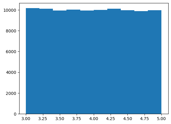
uniform()

It generates random numbers between the specified low and high values (inclusive for low and exclusive for high) using the format: random.uniform(low=0.0, high=1.0, size=None).

• size is the shape of the output array containing the randomly chosen values.

The numbers are selected from a uniform distribution, meaning every value within the specified range has an equal probability of being chosen.

The following code generates a single random number between 0 and 1:

np.random.uniform()

0.4833583569901593

10 random numbers between 5 and 7:

np.random.uniform(5,7,10)

array([6.93958109, 5.9098756 , 6.71902334, 6.87653921, 5.66234391,
       6.31633581, 5.3674959 , 6.62699153, 5.21734002, 6.07325553])

The following code generates a 2D array with 2 rows and 3 columns filled with random numbers between 5 and 7:

np.random.uniform(5,7,(2,3))

array([[5.66793726, 5.48120079, 6.46718961],
       [5.18870794, 6.94859288, 5.650964  ]])

normal()

The function generates random numbers from a normal (Gaussian) distribution based on the specified mean (loc) and standard deviation (scale) values, using the format: random.normal(loc=0.0, scale=1.0, size=None).

Unlike uniform distribution, where every value within a range has an equal chance of being selected, in a normal distribution, values closer to the mean are more likely to be chosen. This reflects the bell-shaped curve characteristic of the normal distribution.

The code below generates a single random number from a normal distribution with a mean of 0 and a standard deviation of 1:

np.random.normal()

0.31374383274018963

10 random numbers chosen from a normal distribution with a mean of 0 and a standard deviation of 1:

np.random.uniform(0,1,10)

array([0.94268858, 0.0792644 , 0.94616421, 0.65958059, 0.91852409,
       0.71114999, 0.35884285, 0.16633063, 0.65666641, 0.95769996])

The following code generates a 2D array with 2 rows and 3 columns filled with random numbers chosen from a normal distribution with a mean of 0 and a standard deviation of 1:

np.random.normal(size=(2,3))

array([[ 0.65196966, -0.35802709,  0.04019786],
       [-0.26987366,  0.83463569,  1.49766058]])

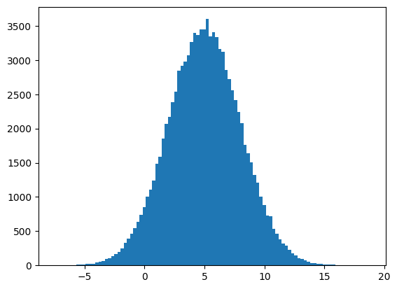
In the following code, we plot a histogram of 10,000 random numbers selected from a normal distribution with a mean of 5 and a standard deviation of 3.

• Most of the points are concentrated around the mean (5):

import matplotlib.pyplot as plt
plt.hist(np.random.normal(5,3,100_000), bins=100);

choice()

This method generates a random sample for the given size from a 1-D array using the format: random.choice(a, size=None, replace=True, p=None).

• If replace=False, the values can not berepeated in the array, as each value is chosen randomly with ensuring that it is unique.

• However, if replace=True, the same value can be selected multiple times.

In the following code, an array of size (2, 3) is generated by choosing random values from [‘a’, ‘b’, ‘c’, ‘d’, ‘e’]:

np.random.choice(['a', 'b', 'c', 'd', 'e'], size=(2,3))

array([['c', 'b', 'a'],
       ['e', 'a', 'a']], dtype='<U1')

In the following code, an array of size (2, 2) is generated by choosing random values from [‘a’, ‘b’, ‘c’, ‘d’, ‘e’] without repetition:

np.random.choice(['a', 'b', 'c', 'd', 'e'], replace=False, size=(2,2))

array([['d', 'c'],
       ['b', 'a']], dtype='<U1')

seed()

Random numbers in the np.random module are generated using a seed, which is a number specified in the format random.seed(seed=None). You can think of the seed as the starting point for generating random numbers.

• By default, if you run the code multiple times, you will get different random numbers because a different seed is chosen each time, which affects the randomly selected values.

• If you want to obtain the same result each time you run the code, you can fix the seed. By setting a fixed seed value, you will ensure that the random numbers generated are the same every time you run the code.

In the following code, every time you run it, you will get a different value:

np.random.uniform()

0.5327401753473313

However, if you set a fixed seed at the beginning you will get the same result every time you run the code below:

np.random.seed(0)
np.random.uniform()

0.5488135039273248

Images

Images can be stored as ndarrays and modified using array methods.

2-Dimensional Images

matplotlib.pyplot is used to plot images.

• By default, the colormap is viridis (yellow-blue).

  • The smallest number in the ndarray corresponds to blue, while the largest represents yellow.

  • For additional colormap options, refer to the following link: colormaps

  • In gray colormap, the smallest number in the ndarray represents black, and the largest one represents white.

myarray = np.array([[1,4,7,10,1]])

For the given ndarray above and the viridis colormap:

• The largest number, 10, corresponds to yellow.

• The smallest number, 1, corresponds to (dark) blue

import matplotlib.pyplot as plt
plt.imshow(myarray)
plt.axis('off');  # remove axis

For the given ndarray above and the gray colormap:

• The largest number, 10, corresponds to white.

• The smallest number, 1, corresponds to black

plt.imshow(myarray, 'gray')
plt.axis('off');  # remove axis

# 1: yellow
# 2: blue
myarray = np.array([[1,0], [0,1]])
plt.figure(figsize=(3,3))
plt.imshow(myarray)
plt.axis('off');  # remove axis

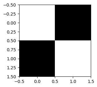
# 1: white
# 2: black
myarray = np.array([[1,0], [0,1]])
plt.figure(figsize=(3,3))
plt.imshow(myarray, 'gray');

Digits Dataset

The digits dataset in sklearn library consists of 1797 pictures of handwritten digits.

• Each picture is represented as an 8 by 8 pixel image, resulting in relatively low picture quality.

We import load_digits() from sklearn.datasets module

• Its type is Bunch, which is similar to dictionaries.

from sklearn.datasets import load_digits
dataset = load_digits()
print(type(dataset))

<class 'sklearn.utils._bunch.Bunch'>

• The images are in the value correspond to the key images.

• You can also use the key DESCR as follows, to access more about the dataset.

print(dataset.DESCR)

print(dataset.keys())

dict_keys(['data', 'target', 'frame', 'feature_names', 'target_names', 'images', 'DESCR'])

• There are 1797 images in this dataset.

• Each picture is represented by an 8 by 8 ndarray.

print(dataset.images.shape)

(1797, 8, 8)

• The first image in the dataset:

image0  = dataset.images[0]
print(image0.shape)

(8, 8)

print(image0)

[[ 0.  0.  5. 13.  9.  1.  0.  0.]
 [ 0.  0. 13. 15. 10. 15.  5.  0.]
 [ 0.  3. 15.  2.  0. 11.  8.  0.]
 [ 0.  4. 12.  0.  0.  8.  8.  0.]
 [ 0.  5.  8.  0.  0.  9.  8.  0.]
 [ 0.  4. 11.  0.  1. 12.  7.  0.]
 [ 0.  2. 14.  5. 10. 12.  0.  0.]
 [ 0.  0.  6. 13. 10.  0.  0.  0.]]

plt.figure(figsize=(1,1))
plt.imshow(image0, 'gray')
plt.axis('off');

• The second image in the dataset.

image1  = dataset.images[1]
print(image1.shape)

(8, 8)

plt.figure(figsize=(1,1))
plt.imshow(image1, 'gray')
plt.axis('off');

Face Dataset

The fetch_lfw_people dataset contains images of famous individuals.

• The parameter min_faces_per_person determines the inclusion of images for individuals who have more than the specified number of pictures in the dataset.

from sklearn.datasets import fetch_lfw_people
dataset = fetch_lfw_people(min_faces_per_person=50)

print(dataset.keys())

dict_keys(['data', 'images', 'target', 'target_names', 'DESCR'])

• There are 1560 images in this dataset.

• Each picture is represented by an 62 by 47 ndarray.

print(dataset.images.shape)

(1560, 62, 47)

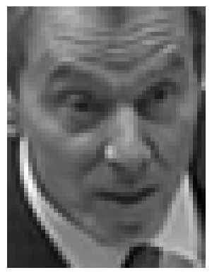
• The first image in the dataset:

image0  = dataset.images[0]
print(image0.shape)

(62, 47)

print(image0)

[[0.3150327  0.33333334 0.39738563 ... 0.22352941 0.2784314  0.30588236]
 [0.3385621  0.34901962 0.40392157 ... 0.15555556 0.22745098 0.3124183 ]
 [0.36078432 0.38039216 0.37124184 ... 0.17254902 0.18431373 0.2496732 ]
 ...
 [0.18692811 0.18431373 0.1751634  ... 0.6640523  0.4366013  0.3124183 ]
 [0.18692811 0.18954249 0.18169935 ... 0.58300656 0.54640526 0.3895425 ]
 [0.18692811 0.18562092 0.18039216 ... 0.5254902  0.606536   0.46535948]]

• The target of the first image is 11.

  • This is the index of the name of the person in target names.

print(dataset.target[0])

11

• This image belongs to Tony Blair.

dataset.target_names[11]

'Tony Blair'

plt.imshow(image0, 'gray')
plt.axis('off');