DataFrames Advanced Methods

import pandas as pd

The following dataframes will be used throughout this section.

df1 = pd.DataFrame({'1C1':[3,4,5], '1C2':[30,40,50], 'col':[300,400,500]}, index=['A', 'B', 'C'])
df1

	1C1	1C2	col
A	3	30	300
B	4	40	400
C	5	50	500

df2 = pd.DataFrame({'2C1':[5,6,9], '2C2':[50,60,90]}, index=['A', 'B', 'C'])
df2

	2C1	2C2
A	5	50
B	6	60
C	9	90

df3 = pd.DataFrame({'3C1':[7,8], '3C2':[70,80], 'col':[700,800]}, index=['C', 'D'])
df3

	3C1	3C2	col
C	7	70	700
D	8	80	800

concat()

It is used to concatenate dataframes along an axis (horizontally or vertically).

# default axis=0: add as new rows
# two new rows coming from df3: C and D
pd.concat([df1,df3])        

	1C1	1C2	col	3C1	3C2
A	3.0	30.0	300	NaN	NaN
B	4.0	40.0	400	NaN	NaN
C	5.0	50.0	500	NaN	NaN
C	NaN	NaN	700	7.0	70.0
D	NaN	NaN	800	8.0	80.0

# axis=1, add as new columns
# three more rows are coming from df3: 3C1, 3C2, col 
pd.concat([df1,df3], axis=1)   

	1C1	1C2	col	3C1	3C2	col
A	3.0	30.0	300.0	NaN	NaN	NaN
B	4.0	40.0	400.0	NaN	NaN	NaN
C	5.0	50.0	500.0	7.0	70.0	700.0
D	NaN	NaN	NaN	8.0	80.0	800.0

# along only on common columns
pd.concat([df1,df2], join='inner')   # intersection of columns

A
B
C
A
B
C

• If the indexes of two dataframes are the same, the column labels are different, and axis=1, then the second dataframe is concatenated horizontally.

# default axis=1: add as a new row
pd.concat([df1,df2], axis=1) 

	1C1	1C2	col	2C1	2C2
A	3	30	300	5	50
B	4	40	400	6	60
C	5	50	500	9	90

shift()

It is used to shift the data up or down.

df = pd.DataFrame(['A', 'B', 'C', 'D', 'E'])
df

	0
0	A
1	B
2	C
3	D
4	E

# shift the values down by 1 row
df.shift()

	0
0	None
1	A
2	B
3	C
4	D

# shift the values down by 2 rows
df.shift(2)

	0
0	None
1	None
2	A
3	B
4	C

# shift the values up by 1 row
df.shift(-1)

	0
0	B
1	C
2	D
3	E
4	None

# shift the values up by 2 rows
df.shift(-2)

	0
0	C
1	D
2	E
3	None
4	None

pct_change()

Percentage change between the current and a prior value.

df = pd.DataFrame([500, 400, 600, 150, 180])
df

	0
0	500
1	400
2	600
3	150
4	180

df.pct_change()

	0
0	NaN
1	-0.20
2	0.50
3	-0.75
4	0.20

rolling()

It is used to do calculations using a rolling window.

• The most commonly used methods following the rolling() method are sum(), mean(), median(), and std().

df

	0
0	500
1	400
2	600
3	150
4	180

• rolling() returns a Rolling object.

• The window parameter specifies the size of the moving window and must be provided.

# window=3
type(df.rolling(3))

pandas.core.window.rolling.Rolling

df.rolling(window=3).sum()

	0
0	NaN
1	NaN
2	1500.0
3	1150.0
4	930.0

With a moving window size of 3, the row triplets and corresponding values are as follows:

• Rows 0, 1, and 2: The sum of 500, 400, and 600 is 1500.

• Rows 1, 2, and 3: The sum of 400, 600, and 150 is 1150.

• Rows 2, 3, and 4: The sum of 600, 150, and 180 is 930.

The first two rolling sum values are NaN (not a number) because a minimum of 3 values is required to compute the sum

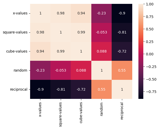
corr()

It returns the correlation coefficients of all column pairs.

Let’s find the correlation coefficients for the following DataFrame.

df4 = pd.DataFrame( {'x-values': [1,2,3,4,5], 'square-values': [1,4,9,16,25],'cube-values': [1,8,27,64,125],
                    'random':[9,4,3,1,8], 'reciprocal': [1/1,1/2,1/3,1/4,1/5]})
df4

	x-values	square-values	cube-values	random	reciprocal
0	1	1	1	9	1.000000
1	2	4	8	4	0.500000
2	3	9	27	3	0.333333
3	4	16	64	1	0.250000
4	5	25	125	8	0.200000

df4.corr()

	x-values	square-values	cube-values	random	reciprocal
x-values	1.000000	0.981105	0.943118	-0.233126	-0.901754
square-values	0.981105	1.000000	0.989216	-0.053368	-0.806339
cube-values	0.943118	0.989216	1.000000	0.088235	-0.722074
random	-0.233126	-0.053368	0.088235	1.000000	0.553018
reciprocal	-0.901754	-0.806339	-0.722074	0.553018	1.000000

The correlation matrix can be visualized using Seaborn’s heatmap function.

import seaborn as sns
sns.heatmap(df4.corr(), annot=True);

groupby()

The groupby() function is used to group rows based on column values.

• It is commonly used to apply functions, such as calculating the sum, to each group.

df5 = pd.DataFrame({'gender':['M','F','F','M','F'], 'age':[35, 50, 25, 30, 40]})
df5

	gender	age
0	M	35
1	F	50
2	F	25
3	M	30
4	F	40

• The groupby() method below returns a GroupBy object with two groups, corresponding to ‘M’ and ‘F’.

df5.groupby('gender')

<pandas.core.groupby.generic.DataFrameGroupBy object at 0x124ae3d90>

• The sum() method below calculates the total of the age values for the ‘M’ and ‘F’ groups.

df5.groupby('gender').sum()

	age
gender
F	115
M	65

• The mean() method below calculates the mean of the age values for the ‘M’ and ‘F’ groups.

df5.groupby('gender').mean()

	age
gender
F	38.333333
M	32.500000

• The count() method below determines the number of samples (rows) in the ‘M’ and ‘F’ groups.

df5.groupby('gender').count()

	age
gender
F	3
M	2

agg()

The agg() methodapplies specified functions to values along a given axis.

• Syntax: pd.agg(function, axis=0)

df = pd.DataFrame([[7,2], [3,4], [5,6]], columns=['A', 'B'])
df

	A	B
0	7	2
1	3	4
2	5	6

df.agg('sum')

A    15
B    12
dtype: int64

df.agg('sum', axis=1)

0     9
1     7
2    11
dtype: int64

df.agg(['sum', 'min'])

	A	B
sum	15	12
min	3	2

df.agg(lambda x: x**2)

	A	B
0	49	4
1	9	16
2	25	36

df

	A	B
0	7	2
1	3	4
2	5	6

iterrows()

The iterrows() method iterates through the rows of a DataFrame, returning each row as an (index, Series) pair.

• It returns a generator object.

• The index represents the row index in the DataFrame.

df.iterrows()

<generator object DataFrame.iterrows at 0x13480ace0>

list(df.iterrows())

[(0,
  A    7
  B    2
  Name: 0, dtype: int64),
 (1,
  A    3
  B    4
  Name: 1, dtype: int64),
 (2,
  A    5
  B    6
  Name: 2, dtype: int64)]

list(df.iloc[1:,:].iterrows())

[(1,
  A    3
  B    4
  Name: 1, dtype: int64),
 (2,
  A    5
  B    6
  Name: 2, dtype: int64)]

for idx, row in df.iterrows():
    print(idx, row.values)

0 [7 2]
1 [3 4]
2 [5 6]

apply()

The apply() method is used to apply a function to either rows or columns of a DataFrame.

• Syntax: df.apply(function, axis=0)

• The default value of axis is 0, meaning the function is applied to each column.

• If axis=1, the function is applied to each row.

• Additionally, a lambda function can be used within apply() to define the function inline.

We will use the apply() method on the following DataFrame.

df

	A	B
0	7	2
1	3	4
2	5	6

In the following example, a custom square function is used to compute the square of values in each column.

def square_function(x):
    return x**2

df.apply(square_function)

	A	B
0	49	4
1	9	16
2	25	36

In the following example, a lambda function is used to define the square function.

df.apply(lambda x: x**2)

	A	B
0	49	4
1	9	16
2	25	36

In the following example, the sum() function from NumPy is used to compute the sum of values in each column.

import numpy as np
df.apply(np.sum)

A    15
B    12
dtype: int64

In the following example, the sum() function from NumPy is used to compute the sum of values in each row.

df.apply(np.sum, axis=1)

0     9
1     7
2    11
dtype: int64

The following example calculates the weighted sum of particular DataFrame columns using a custom function and a lambda function.

def add_weighted_columns(row):
    return 0.2*row['A'] + 0.8*row['B']

df.apply(add_weighted_columns, axis=1)

0    3.0
1    3.8
2    5.8
dtype: float64

df.apply(lambda  row: 0.2*row['A'] + 0.8*row['B'], axis=1)

0    3.0
1    3.8
2    5.8
dtype: float64

at()

The at() method is used to access a single value from a DataFrame using a specific row and column label pair.

It is similar to loc, but at() is used for retrieving a single value and does not support slicing.

df

	A	B
0	7	2
1	3	4
2	5	6

df.at[1,'B']

4