Datasets#

Sklearn In-Built Datasets#
Certain Python libraries/packages offer built-in datasets that can be used for prectices.
Different libraries or packages may return datasets in various formats.
This section will introduce some of the datasets available in Sklearn.
Iris Dataset#
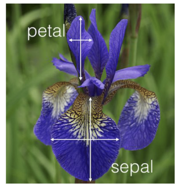
The Iris dataset consists of petal and sepal width-length measurements of 150 iris flowers.
There are 50 samples from each of the following three species (classes):
Setosa
Versicolor
Virginica
It is used for classification tasks in data analysis, as the flower classes are given.
picture sourced from https://www.uvm.edu/~rsingle/stat3880/S24/notes/ch4-5_LDA-IrisData.pdf
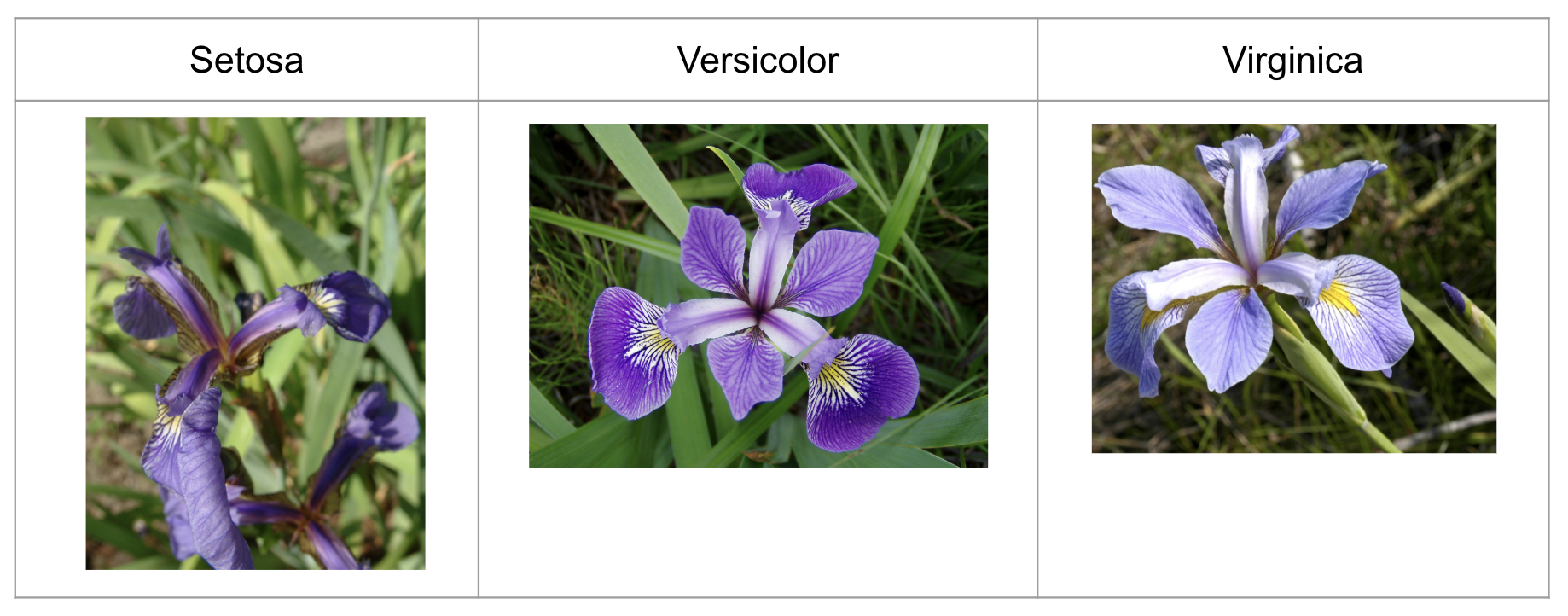
picture sourced from https://en.wikipedia.org/wiki/Iris_flower_data_set
load_iris()#
The load_iris function is imported from sklearn.datasets.
load_iris() returns a Bunch object, which is similar to a dictionary.
The keys of a Bunch object can be accessed using dot notation (e.g., load_iris().key_name) as well as square bracket notation (e.g., load_iris[‘key_name’]) like dictionaries.
from sklearn.datasets import load_iris
# load_iris is a function
type(load_iris)
function
# iris is a bunch
iris = load_iris()
type(iris)
sklearn.utils._bunch.Bunch
keys()#
It returns the keys of the Bunch object iris.
iris.keys()
dict_keys(['data', 'target', 'frame', 'target_names', 'DESCR', 'feature_names', 'filename', 'data_module'])
DESCR#
The DESCR attribute provides a detailed description of the dataset as a string.
Use the print() function to render it in a more readable format.
type(iris.DESCR)
str
# not easy to read
iris.DESCR
'.. _iris_dataset:\n\nIris plants dataset\n--------------------\n\n**Data Set Characteristics:**\n\n:Number of Instances: 150 (50 in each of three classes)\n:Number of Attributes: 4 numeric, predictive attributes and the class\n:Attribute Information:\n - sepal length in cm\n - sepal width in cm\n - petal length in cm\n - petal width in cm\n - class:\n - Iris-Setosa\n - Iris-Versicolour\n - Iris-Virginica\n\n:Summary Statistics:\n\n============== ==== ==== ======= ===== ====================\n Min Max Mean SD Class Correlation\n============== ==== ==== ======= ===== ====================\nsepal length: 4.3 7.9 5.84 0.83 0.7826\nsepal width: 2.0 4.4 3.05 0.43 -0.4194\npetal length: 1.0 6.9 3.76 1.76 0.9490 (high!)\npetal width: 0.1 2.5 1.20 0.76 0.9565 (high!)\n============== ==== ==== ======= ===== ====================\n\n:Missing Attribute Values: None\n:Class Distribution: 33.3% for each of 3 classes.\n:Creator: R.A. Fisher\n:Donor: Michael Marshall (MARSHALL%PLU@io.arc.nasa.gov)\n:Date: July, 1988\n\nThe famous Iris database, first used by Sir R.A. Fisher. The dataset is taken\nfrom Fisher\'s paper. Note that it\'s the same as in R, but not as in the UCI\nMachine Learning Repository, which has two wrong data points.\n\nThis is perhaps the best known database to be found in the\npattern recognition literature. Fisher\'s paper is a classic in the field and\nis referenced frequently to this day. (See Duda & Hart, for example.) The\ndata set contains 3 classes of 50 instances each, where each class refers to a\ntype of iris plant. One class is linearly separable from the other 2; the\nlatter are NOT linearly separable from each other.\n\n.. dropdown:: References\n\n - Fisher, R.A. "The use of multiple measurements in taxonomic problems"\n Annual Eugenics, 7, Part II, 179-188 (1936); also in "Contributions to\n Mathematical Statistics" (John Wiley, NY, 1950).\n - Duda, R.O., & Hart, P.E. (1973) Pattern Classification and Scene Analysis.\n (Q327.D83) John Wiley & Sons. ISBN 0-471-22361-1. See page 218.\n - Dasarathy, B.V. (1980) "Nosing Around the Neighborhood: A New System\n Structure and Classification Rule for Recognition in Partially Exposed\n Environments". IEEE Transactions on Pattern Analysis and Machine\n Intelligence, Vol. PAMI-2, No. 1, 67-71.\n - Gates, G.W. (1972) "The Reduced Nearest Neighbor Rule". IEEE Transactions\n on Information Theory, May 1972, 431-433.\n - See also: 1988 MLC Proceedings, 54-64. Cheeseman et al"s AUTOCLASS II\n conceptual clustering system finds 3 classes in the data.\n - Many, many more ...\n'
print(iris.DESCR[:])
.. _iris_dataset:

Iris plants dataset
--------------------

**Data Set Characteristics:**

:Number of Instances: 150 (50 in each of three classes)
:Number of Attributes: 4 numeric, predictive attributes and the class
:Attribute Information:
    - sepal length in cm
    - sepal width in cm
    - petal length in cm
    - petal width in cm
    - class:
            - Iris-Setosa
            - Iris-Versicolour
            - Iris-Virginica

:Summary Statistics:

============== ==== ==== ======= ===== ====================
                Min  Max   Mean    SD   Class Correlation
============== ==== ==== ======= ===== ====================
sepal length:   4.3  7.9   5.84   0.83    0.7826
sepal width:    2.0  4.4   3.05   0.43   -0.4194
petal length:   1.0  6.9   3.76   1.76    0.9490  (high!)
petal width:    0.1  2.5   1.20   0.76    0.9565  (high!)
============== ==== ==== ======= ===== ====================

:Missing Attribute Values: None
:Class Distribution: 33.3% for each of 3 classes.
:Creator: R.A. Fisher
:Donor: Michael Marshall (MARSHALL%PLU@io.arc.nasa.gov)
:Date: July, 1988

The famous Iris database, first used by Sir R.A. Fisher. The dataset is taken
from Fisher's paper. Note that it's the same as in R, but not as in the UCI
Machine Learning Repository, which has two wrong data points.

This is perhaps the best known database to be found in the
pattern recognition literature.  Fisher's paper is a classic in the field and
is referenced frequently to this day.  (See Duda & Hart, for example.)  The
data set contains 3 classes of 50 instances each, where each class refers to a
type of iris plant.  One class is linearly separable from the other 2; the
latter are NOT linearly separable from each other.

.. dropdown:: References

  - Fisher, R.A. "The use of multiple measurements in taxonomic problems"
    Annual Eugenics, 7, Part II, 179-188 (1936); also in "Contributions to
    Mathematical Statistics" (John Wiley, NY, 1950).
  - Duda, R.O., & Hart, P.E. (1973) Pattern Classification and Scene Analysis.
    (Q327.D83) John Wiley & Sons.  ISBN 0-471-22361-1.  See page 218.
  - Dasarathy, B.V. (1980) "Nosing Around the Neighborhood: A New System
    Structure and Classification Rule for Recognition in Partially Exposed
    Environments".  IEEE Transactions on Pattern Analysis and Machine
    Intelligence, Vol. PAMI-2, No. 1, 67-71.
  - Gates, G.W. (1972) "The Reduced Nearest Neighbor Rule".  IEEE Transactions
    on Information Theory, May 1972, 431-433.
  - See also: 1988 MLC Proceedings, 54-64.  Cheeseman et al"s AUTOCLASS II
    conceptual clustering system finds 3 classes in the data.
  - Many, many more ...
data#
The data attribute returns a NumPy array. It serves as the input data for modeling tasks.
It contains four measurements (sepal length, sepal width, petal length, petal width) for each flower.
Its shape is 150 by 4.
150 samples (flowers)
4 features (measurements)
iris.data[:3]
array([[5.1, 3.5, 1.4, 0.2],
       [4.9, 3. , 1.4, 0.2],
       [4.7, 3.2, 1.3, 0.2]])
iris.data.shape
(150, 4)
target#
The target attribute returns a NumPy array. It serves as the output data for modeling tasks.
It consists of the types/classes/species of each flower.
Its shape is (150,)
150 samples (flowers)
The three classes—Setosa, Versicolor, and Virginica—are represented by the numbers 0, 1, and 2, respectively.
iris.target
array([0, 0, 0, 0, 0, 0, 0, 0, 0, 0, 0, 0, 0, 0, 0, 0, 0, 0, 0, 0, 0, 0,
       0, 0, 0, 0, 0, 0, 0, 0, 0, 0, 0, 0, 0, 0, 0, 0, 0, 0, 0, 0, 0, 0,
       0, 0, 0, 0, 0, 0, 1, 1, 1, 1, 1, 1, 1, 1, 1, 1, 1, 1, 1, 1, 1, 1,
       1, 1, 1, 1, 1, 1, 1, 1, 1, 1, 1, 1, 1, 1, 1, 1, 1, 1, 1, 1, 1, 1,
       1, 1, 1, 1, 1, 1, 1, 1, 1, 1, 1, 1, 2, 2, 2, 2, 2, 2, 2, 2, 2, 2,
       2, 2, 2, 2, 2, 2, 2, 2, 2, 2, 2, 2, 2, 2, 2, 2, 2, 2, 2, 2, 2, 2,
       2, 2, 2, 2, 2, 2, 2, 2, 2, 2, 2, 2, 2, 2, 2, 2, 2, 2])
iris.target.shape
(150,)
target_names#
It returns the names of the three classes that are represented by numbers in the target.
iris.target_names
array(['setosa', 'versicolor', 'virginica'], dtype='<U10')
feature_names#
It returns the names of the four features (measurements).
iris.feature_names
['sepal length (cm)',
 'sepal width (cm)',
 'petal length (cm)',
 'petal width (cm)']
California Housing Dataset#
The California Housing dataset contains housing information for 20,640 districts in California.
It is used for regression tasks in data analysis.
from sklearn.datasets import fetch_california_housing
fetch_california_housing()#
The fetch_california_housing function is imported from sklearn.datasets.
fetch_california_housing() returns a Bunch object, which is similar to a dictionary.
The keys of a Bunch object can be accessed using dot notation (e.g., fetch_california_housing().key_name) as well as square bracket notation (e.g., lfetch_california_housing[‘key_name’]) like dictionaries.
housing = fetch_california_housing()
keys()#
It returns the keys of the Bunch object housing.
housing.keys()
dict_keys(['data', 'target', 'frame', 'target_names', 'feature_names', 'DESCR'])
DESCR#
The DESCR attribute provides a detailed description of the dataset as a string.
Use the print() function to render it in a more readable format.
housing.DESCR
'.. _california_housing_dataset:\n\nCalifornia Housing dataset\n--------------------------\n\n**Data Set Characteristics:**\n\n:Number of Instances: 20640\n\n:Number of Attributes: 8 numeric, predictive attributes and the target\n\n:Attribute Information:\n - MedInc median income in block group\n - HouseAge median house age in block group\n - AveRooms average number of rooms per household\n - AveBedrms average number of bedrooms per household\n - Population block group population\n - AveOccup average number of household members\n - Latitude block group latitude\n - Longitude block group longitude\n\n:Missing Attribute Values: None\n\nThis dataset was obtained from the StatLib repository.\nhttps://www.dcc.fc.up.pt/~ltorgo/Regression/cal_housing.html\n\nThe target variable is the median house value for California districts,\nexpressed in hundreds of thousands of dollars ($100,000).\n\nThis dataset was derived from the 1990 U.S. census, using one row per census\nblock group. A block group is the smallest geographical unit for which the U.S.\nCensus Bureau publishes sample data (a block group typically has a population\nof 600 to 3,000 people).\n\nA household is a group of people residing within a home. Since the average\nnumber of rooms and bedrooms in this dataset are provided per household, these\ncolumns may take surprisingly large values for block groups with few households\nand many empty houses, such as vacation resorts.\n\nIt can be downloaded/loaded using the\n:func:`sklearn.datasets.fetch_california_housing` function.\n\n.. rubric:: References\n\n- Pace, R. Kelley and Ronald Barry, Sparse Spatial Autoregressions,\n Statistics and Probability Letters, 33 (1997) 291-297\n'
print(housing.DESCR)
.. _california_housing_dataset:

California Housing dataset
--------------------------

**Data Set Characteristics:**

:Number of Instances: 20640

:Number of Attributes: 8 numeric, predictive attributes and the target

:Attribute Information:
    - MedInc        median income in block group
    - HouseAge      median house age in block group
    - AveRooms      average number of rooms per household
    - AveBedrms     average number of bedrooms per household
    - Population    block group population
    - AveOccup      average number of household members
    - Latitude      block group latitude
    - Longitude     block group longitude

:Missing Attribute Values: None

This dataset was obtained from the StatLib repository.
https://www.dcc.fc.up.pt/~ltorgo/Regression/cal_housing.html

The target variable is the median house value for California districts,
expressed in hundreds of thousands of dollars ($100,000).

This dataset was derived from the 1990 U.S. census, using one row per census
block group. A block group is the smallest geographical unit for which the U.S.
Census Bureau publishes sample data (a block group typically has a population
of 600 to 3,000 people).

A household is a group of people residing within a home. Since the average
number of rooms and bedrooms in this dataset are provided per household, these
columns may take surprisingly large values for block groups with few households
and many empty houses, such as vacation resorts.

It can be downloaded/loaded using the
:func:`sklearn.datasets.fetch_california_housing` function.

.. rubric:: References

- Pace, R. Kelley and Ronald Barry, Sparse Spatial Autoregressions,
  Statistics and Probability Letters, 33 (1997) 291-297
data#
The data attribute returns a NumPy array. It serves as the input data for modeling tasks.
It contains eight features (MedInc, HouseAge, AveRooms, AveBedrms, Population, AveOccup, Latitude, Longitude) for each block.
Its shape is 20640 by 8.
20640 samples (blocks)
8 features
housing.data[:2]
array([[ 8.32520000e+00,  4.10000000e+01,  6.98412698e+00,
         1.02380952e+00,  3.22000000e+02,  2.55555556e+00,
         3.78800000e+01, -1.22230000e+02],
       [ 8.30140000e+00,  2.10000000e+01,  6.23813708e+00,
         9.71880492e-01,  2.40100000e+03,  2.10984183e+00,
         3.78600000e+01, -1.22220000e+02]])
housing.data.shape
(20640, 8)
target#
The target attribute returns a NumPy array. It serves as the output data for modeling tasks.
It consists of the median house value of each block.
Its shape is (20640,)
20640 samples (blocks)
housing.target
array([4.526, 3.585, 3.521, ..., 0.923, 0.847, 0.894])
housing.target.shape
(20640,)
target_names#
It returns the names of the outputs that are in the target.
housing.target_names
['MedHouseVal']
feature_names#
It returns the names of the eight features.
housing.feature_names
['MedInc',
 'HouseAge',
 'AveRooms',
 'AveBedrms',
 'Population',
 'AveOccup',
 'Latitude',
 'Longitude']
Digits Dataset#
The Digits dataset consists of 8x8 pixel images of 1797 handwritten digits.
It is used for classification tasks in data analysis, as the actual digit classes are given.
load_digits()#
The load_digits function is imported from sklearn.datasets.
load_digits() returns a Bunch object, which is similar to a dictionary.
The keys of a Bunch object can be accessed using dot notation (e.g., load_digits().key_name) as well as square bracket notation (e.g., load_digits[‘key_name’]) like dictionaries.
from sklearn.datasets import load_digits
# load_digits is a function
type(load_digits)
function
# digits is a bunch
digits = load_digits()
type(digits)
sklearn.utils._bunch.Bunch
keys()#
It returns the keys of the Bunch object iris.
digits.keys()
dict_keys(['data', 'target', 'frame', 'feature_names', 'target_names', 'images', 'DESCR'])
DESCR#
The DESCR attribute provides a detailed description of the dataset as a string.
Use the print() function to render it in a more readable format.
type(digits.DESCR)
str
# not easy to read
digits.DESCR
".. _digits_dataset:\n\nOptical recognition of handwritten digits dataset\n--------------------------------------------------\n\n**Data Set Characteristics:**\n\n:Number of Instances: 1797\n:Number of Attributes: 64\n:Attribute Information: 8x8 image of integer pixels in the range 0..16.\n:Missing Attribute Values: None\n:Creator: E. Alpaydin (alpaydin '@' boun.edu.tr)\n:Date: July; 1998\n\nThis is a copy of the test set of the UCI ML hand-written digits datasets\nhttps://archive.ics.uci.edu/ml/datasets/Optical+Recognition+of+Handwritten+Digits\n\nThe data set contains images of hand-written digits: 10 classes where\neach class refers to a digit.\n\nPreprocessing programs made available by NIST were used to extract\nnormalized bitmaps of handwritten digits from a preprinted form. From a\ntotal of 43 people, 30 contributed to the training set and different 13\nto the test set. 32x32 bitmaps are divided into nonoverlapping blocks of\n4x4 and the number of on pixels are counted in each block. This generates\nan input matrix of 8x8 where each element is an integer in the range\n0..16. This reduces dimensionality and gives invariance to small\ndistortions.\n\nFor info on NIST preprocessing routines, see M. D. Garris, J. L. Blue, G.\nT. Candela, D. L. Dimmick, J. Geist, P. J. Grother, S. A. Janet, and C.\nL. Wilson, NIST Form-Based Handprint Recognition System, NISTIR 5469,\n1994.\n\n.. dropdown:: References\n\n - C. Kaynak (1995) Methods of Combining Multiple Classifiers and Their\n Applications to Handwritten Digit Recognition, MSc Thesis, Institute of\n Graduate Studies in Science and Engineering, Bogazici University.\n - E. Alpaydin, C. Kaynak (1998) Cascading Classifiers, Kybernetika.\n - Ken Tang and Ponnuthurai N. Suganthan and Xi Yao and A. Kai Qin.\n Linear dimensionalityreduction using relevance weighted LDA. School of\n Electrical and Electronic Engineering Nanyang Technological University.\n 2005.\n - Claudio Gentile. A New Approximate Maximal Margin Classification\n Algorithm. NIPS. 2000.\n"
print(digits.DESCR)
.. _digits_dataset:

Optical recognition of handwritten digits dataset
--------------------------------------------------

**Data Set Characteristics:**

:Number of Instances: 1797
:Number of Attributes: 64
:Attribute Information: 8x8 image of integer pixels in the range 0..16.
:Missing Attribute Values: None
:Creator: E. Alpaydin (alpaydin '@' boun.edu.tr)
:Date: July; 1998

This is a copy of the test set of the UCI ML hand-written digits datasets
https://archive.ics.uci.edu/ml/datasets/Optical+Recognition+of+Handwritten+Digits

The data set contains images of hand-written digits: 10 classes where
each class refers to a digit.

Preprocessing programs made available by NIST were used to extract
normalized bitmaps of handwritten digits from a preprinted form. From a
total of 43 people, 30 contributed to the training set and different 13
to the test set. 32x32 bitmaps are divided into nonoverlapping blocks of
4x4 and the number of on pixels are counted in each block. This generates
an input matrix of 8x8 where each element is an integer in the range
0..16. This reduces dimensionality and gives invariance to small
distortions.

For info on NIST preprocessing routines, see M. D. Garris, J. L. Blue, G.
T. Candela, D. L. Dimmick, J. Geist, P. J. Grother, S. A. Janet, and C.
L. Wilson, NIST Form-Based Handprint Recognition System, NISTIR 5469,
1994.

.. dropdown:: References

  - C. Kaynak (1995) Methods of Combining Multiple Classifiers and Their
    Applications to Handwritten Digit Recognition, MSc Thesis, Institute of
    Graduate Studies in Science and Engineering, Bogazici University.
  - E. Alpaydin, C. Kaynak (1998) Cascading Classifiers, Kybernetika.
  - Ken Tang and Ponnuthurai N. Suganthan and Xi Yao and A. Kai Qin.
    Linear dimensionalityreduction using relevance weighted LDA. School of
    Electrical and Electronic Engineering Nanyang Technological University.
    2005.
  - Claudio Gentile. A New Approximate Maximal Margin Classification
    Algorithm. NIPS. 2000.
data#
The data attribute returns a NumPy array. It serves as the input data for modeling tasks.
It contains 64 numbers for each image that represents 8x8 pixels.
Its shape is 1797 by 64.
1797 samples (images)
64 pixels
digits.data[:3]
array([[ 0.,  0.,  5., 13.,  9.,  1.,  0.,  0.,  0.,  0., 13., 15., 10.,
        15.,  5.,  0.,  0.,  3., 15.,  2.,  0., 11.,  8.,  0.,  0.,  4.,
        12.,  0.,  0.,  8.,  8.,  0.,  0.,  5.,  8.,  0.,  0.,  9.,  8.,
         0.,  0.,  4., 11.,  0.,  1., 12.,  7.,  0.,  0.,  2., 14.,  5.,
        10., 12.,  0.,  0.,  0.,  0.,  6., 13., 10.,  0.,  0.,  0.],
       [ 0.,  0.,  0., 12., 13.,  5.,  0.,  0.,  0.,  0.,  0., 11., 16.,
         9.,  0.,  0.,  0.,  0.,  3., 15., 16.,  6.,  0.,  0.,  0.,  7.,
        15., 16., 16.,  2.,  0.,  0.,  0.,  0.,  1., 16., 16.,  3.,  0.,
         0.,  0.,  0.,  1., 16., 16.,  6.,  0.,  0.,  0.,  0.,  1., 16.,
        16.,  6.,  0.,  0.,  0.,  0.,  0., 11., 16., 10.,  0.,  0.],
       [ 0.,  0.,  0.,  4., 15., 12.,  0.,  0.,  0.,  0.,  3., 16., 15.,
        14.,  0.,  0.,  0.,  0.,  8., 13.,  8., 16.,  0.,  0.,  0.,  0.,
         1.,  6., 15., 11.,  0.,  0.,  0.,  1.,  8., 13., 15.,  1.,  0.,
         0.,  0.,  9., 16., 16.,  5.,  0.,  0.,  0.,  0.,  3., 13., 16.,
        16., 11.,  5.,  0.,  0.,  0.,  0.,  3., 11., 16.,  9.,  0.]])
digits.data.shape
(1797, 64)
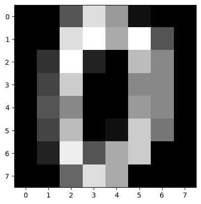
image#
It returns each image as an 8x8 array, allowing it to be displayed as follows:
import matplotlib.pyplot as plt
# first image
plt.imshow(digits.images[0], 'gray');
# smaller size and no axis lines
plt.figure(figsize=(2,2))
plt.imshow(digits.images[0], 'gray')
plt.axis('off');

target#
The target attribute returns a NumPy array. It serves as the output data for modeling tasks.
It consists of the actual class of each image.
Its shape is (1797,)
1797 samples (images)
digits.target
array([0, 1, 2, ..., 8, 9, 8])
digits.target.shape
(1797,)
target_names#
It returns the digits: 0,1,2,3,4,5,6,7,8,9
digits.target_names
array([0, 1, 2, 3, 4, 5, 6, 7, 8, 9])
feature_names#
It returns the names of all pixels.
digits.feature_names
['pixel_0_0',
 'pixel_0_1',
 'pixel_0_2',
 'pixel_0_3',
 'pixel_0_4',
 'pixel_0_5',
 'pixel_0_6',
 'pixel_0_7',
 'pixel_1_0',
 'pixel_1_1',
 'pixel_1_2',
 'pixel_1_3',
 'pixel_1_4',
 'pixel_1_5',
 'pixel_1_6',
 'pixel_1_7',
 'pixel_2_0',
 'pixel_2_1',
 'pixel_2_2',
 'pixel_2_3',
 'pixel_2_4',
 'pixel_2_5',
 'pixel_2_6',
 'pixel_2_7',
 'pixel_3_0',
 'pixel_3_1',
 'pixel_3_2',
 'pixel_3_3',
 'pixel_3_4',
 'pixel_3_5',
 'pixel_3_6',
 'pixel_3_7',
 'pixel_4_0',
 'pixel_4_1',
 'pixel_4_2',
 'pixel_4_3',
 'pixel_4_4',
 'pixel_4_5',
 'pixel_4_6',
 'pixel_4_7',
 'pixel_5_0',
 'pixel_5_1',
 'pixel_5_2',
 'pixel_5_3',
 'pixel_5_4',
 'pixel_5_5',
 'pixel_5_6',
 'pixel_5_7',
 'pixel_6_0',
 'pixel_6_1',
 'pixel_6_2',
 'pixel_6_3',
 'pixel_6_4',
 'pixel_6_5',
 'pixel_6_6',
 'pixel_6_7',
 'pixel_7_0',
 'pixel_7_1',
 'pixel_7_2',
 'pixel_7_3',
 'pixel_7_4',
 'pixel_7_5',
 'pixel_7_6',
 'pixel_7_7']
Wine Dataset#
This dataset consists of data from 178 wine samples, each characterized by 13 features.
It is a classification dataset with three classes: class_0, class_1, and class_2.
from sklearn.datasets import load_wine
# load_breast_cancer is a function
type(load_wine)
function
# wine is a bunch
wine = load_wine()
type(wine)
sklearn.utils._bunch.Bunch
keys()#
It returns the keys of the Bunch object cancer.
wine.keys()
dict_keys(['data', 'target', 'frame', 'target_names', 'DESCR', 'feature_names'])
DESCR#
The DESCR attribute provides a detailed description of the dataset as a string.
Use the print() function to render it in a more readable format.
type(wine.DESCR)
str
# not easy to read
wine.DESCR
'.. _wine_dataset:\n\nWine recognition dataset\n------------------------\n\n**Data Set Characteristics:**\n\n:Number of Instances: 178\n:Number of Attributes: 13 numeric, predictive attributes and the class\n:Attribute Information:\n - Alcohol\n - Malic acid\n - Ash\n - Alcalinity of ash\n - Magnesium\n - Total phenols\n - Flavanoids\n - Nonflavanoid phenols\n - Proanthocyanins\n - Color intensity\n - Hue\n - OD280/OD315 of diluted wines\n - Proline\n - class:\n - class_0\n - class_1\n - class_2\n\n:Summary Statistics:\n\n============================= ==== ===== ======= =====\n Min Max Mean SD\n============================= ==== ===== ======= =====\nAlcohol: 11.0 14.8 13.0 0.8\nMalic Acid: 0.74 5.80 2.34 1.12\nAsh: 1.36 3.23 2.36 0.27\nAlcalinity of Ash: 10.6 30.0 19.5 3.3\nMagnesium: 70.0 162.0 99.7 14.3\nTotal Phenols: 0.98 3.88 2.29 0.63\nFlavanoids: 0.34 5.08 2.03 1.00\nNonflavanoid Phenols: 0.13 0.66 0.36 0.12\nProanthocyanins: 0.41 3.58 1.59 0.57\nColour Intensity: 1.3 13.0 5.1 2.3\nHue: 0.48 1.71 0.96 0.23\nOD280/OD315 of diluted wines: 1.27 4.00 2.61 0.71\nProline: 278 1680 746 315\n============================= ==== ===== ======= =====\n\n:Missing Attribute Values: None\n:Class Distribution: class_0 (59), class_1 (71), class_2 (48)\n:Creator: R.A. Fisher\n:Donor: Michael Marshall (MARSHALL%PLU@io.arc.nasa.gov)\n:Date: July, 1988\n\nThis is a copy of UCI ML Wine recognition datasets.\nhttps://archive.ics.uci.edu/ml/machine-learning-databases/wine/wine.data\n\nThe data is the results of a chemical analysis of wines grown in the same\nregion in Italy by three different cultivators. There are thirteen different\nmeasurements taken for different constituents found in the three types of\nwine.\n\nOriginal Owners:\n\nForina, M. et al, PARVUS -\nAn Extendible Package for Data Exploration, Classification and Correlation.\nInstitute of Pharmaceutical and Food Analysis and Technologies,\nVia Brigata Salerno, 16147 Genoa, Italy.\n\nCitation:\n\nLichman, M. (2013). UCI Machine Learning Repository\n[https://archive.ics.uci.edu/ml]. Irvine, CA: University of California,\nSchool of Information and Computer Science.\n\n.. dropdown:: References\n\n (1) S. Aeberhard, D. Coomans and O. de Vel,\n Comparison of Classifiers in High Dimensional Settings,\n Tech. Rep. no. 92-02, (1992), Dept. of Computer Science and Dept. of\n Mathematics and Statistics, James Cook University of North Queensland.\n (Also submitted to Technometrics).\n\n The data was used with many others for comparing various\n classifiers. The classes are separable, though only RDA\n has achieved 100% correct classification.\n (RDA : 100%, QDA 99.4%, LDA 98.9%, 1NN 96.1% (z-transformed data))\n (All results using the leave-one-out technique)\n\n (2) S. Aeberhard, D. Coomans and O. de Vel,\n "THE CLASSIFICATION PERFORMANCE OF RDA"\n Tech. Rep. no. 92-01, (1992), Dept. of Computer Science and Dept. of\n Mathematics and Statistics, James Cook University of North Queensland.\n (Also submitted to Journal of Chemometrics).\n'
print(wine.DESCR[:])
.. _wine_dataset:

Wine recognition dataset
------------------------

**Data Set Characteristics:**

:Number of Instances: 178
:Number of Attributes: 13 numeric, predictive attributes and the class
:Attribute Information:
    - Alcohol
    - Malic acid
    - Ash
    - Alcalinity of ash
    - Magnesium
    - Total phenols
    - Flavanoids
    - Nonflavanoid phenols
    - Proanthocyanins
    - Color intensity
    - Hue
    - OD280/OD315 of diluted wines
    - Proline
    - class:
        - class_0
        - class_1
        - class_2

:Summary Statistics:

============================= ==== ===== ======= =====
                                Min   Max   Mean     SD
============================= ==== ===== ======= =====
Alcohol:                      11.0  14.8    13.0   0.8
Malic Acid:                   0.74  5.80    2.34  1.12
Ash:                          1.36  3.23    2.36  0.27
Alcalinity of Ash:            10.6  30.0    19.5   3.3
Magnesium:                    70.0 162.0    99.7  14.3
Total Phenols:                0.98  3.88    2.29  0.63
Flavanoids:                   0.34  5.08    2.03  1.00
Nonflavanoid Phenols:         0.13  0.66    0.36  0.12
Proanthocyanins:              0.41  3.58    1.59  0.57
Colour Intensity:              1.3  13.0     5.1   2.3
Hue:                          0.48  1.71    0.96  0.23
OD280/OD315 of diluted wines: 1.27  4.00    2.61  0.71
Proline:                       278  1680     746   315
============================= ==== ===== ======= =====

:Missing Attribute Values: None
:Class Distribution: class_0 (59), class_1 (71), class_2 (48)
:Creator: R.A. Fisher
:Donor: Michael Marshall (MARSHALL%PLU@io.arc.nasa.gov)
:Date: July, 1988

This is a copy of UCI ML Wine recognition datasets.
https://archive.ics.uci.edu/ml/machine-learning-databases/wine/wine.data

The data is the results of a chemical analysis of wines grown in the same
region in Italy by three different cultivators. There are thirteen different
measurements taken for different constituents found in the three types of
wine.

Original Owners:

Forina, M. et al, PARVUS -
An Extendible Package for Data Exploration, Classification and Correlation.
Institute of Pharmaceutical and Food Analysis and Technologies,
Via Brigata Salerno, 16147 Genoa, Italy.

Citation:

Lichman, M. (2013). UCI Machine Learning Repository
[https://archive.ics.uci.edu/ml]. Irvine, CA: University of California,
School of Information and Computer Science.

.. dropdown:: References

    (1) S. Aeberhard, D. Coomans and O. de Vel,
    Comparison of Classifiers in High Dimensional Settings,
    Tech. Rep. no. 92-02, (1992), Dept. of Computer Science and Dept. of
    Mathematics and Statistics, James Cook University of North Queensland.
    (Also submitted to Technometrics).

    The data was used with many others for comparing various
    classifiers. The classes are separable, though only RDA
    has achieved 100% correct classification.
    (RDA : 100%, QDA 99.4%, LDA 98.9%, 1NN 96.1% (z-transformed data))
    (All results using the leave-one-out technique)

    (2) S. Aeberhard, D. Coomans and O. de Vel,
    "THE CLASSIFICATION PERFORMANCE OF RDA"
    Tech. Rep. no. 92-01, (1992), Dept. of Computer Science and Dept. of
    Mathematics and Statistics, James Cook University of North Queensland.
    (Also submitted to Journal of Chemometrics).
data#
The data attribute returns a NumPy array. It serves as the input data for modeling tasks.
It contains 13 measurements for each wine.
Its shape is 178 by 13.
178 samples (wines)
13 features (measurements)
wine.data[:3]
array([[1.423e+01, 1.710e+00, 2.430e+00, 1.560e+01, 1.270e+02, 2.800e+00,
        3.060e+00, 2.800e-01, 2.290e+00, 5.640e+00, 1.040e+00, 3.920e+00,
        1.065e+03],
       [1.320e+01, 1.780e+00, 2.140e+00, 1.120e+01, 1.000e+02, 2.650e+00,
        2.760e+00, 2.600e-01, 1.280e+00, 4.380e+00, 1.050e+00, 3.400e+00,
        1.050e+03],
       [1.316e+01, 2.360e+00, 2.670e+00, 1.860e+01, 1.010e+02, 2.800e+00,
        3.240e+00, 3.000e-01, 2.810e+00, 5.680e+00, 1.030e+00, 3.170e+00,
        1.185e+03]])
wine.data.shape
(178, 13)
target#
The target attribute returns a NumPy array. It serves as the output data for modeling tasks.
It consists of the types/classes of each patient.
Its shape is (178,)
178 samples (wines)
The three classes—class_1, class_2 and class_3—are represented by the numbers 0, 1, and 2, respectively.
wine.target
array([0, 0, 0, 0, 0, 0, 0, 0, 0, 0, 0, 0, 0, 0, 0, 0, 0, 0, 0, 0, 0, 0,
       0, 0, 0, 0, 0, 0, 0, 0, 0, 0, 0, 0, 0, 0, 0, 0, 0, 0, 0, 0, 0, 0,
       0, 0, 0, 0, 0, 0, 0, 0, 0, 0, 0, 0, 0, 0, 0, 1, 1, 1, 1, 1, 1, 1,
       1, 1, 1, 1, 1, 1, 1, 1, 1, 1, 1, 1, 1, 1, 1, 1, 1, 1, 1, 1, 1, 1,
       1, 1, 1, 1, 1, 1, 1, 1, 1, 1, 1, 1, 1, 1, 1, 1, 1, 1, 1, 1, 1, 1,
       1, 1, 1, 1, 1, 1, 1, 1, 1, 1, 1, 1, 1, 1, 1, 1, 1, 1, 1, 1, 2, 2,
       2, 2, 2, 2, 2, 2, 2, 2, 2, 2, 2, 2, 2, 2, 2, 2, 2, 2, 2, 2, 2, 2,
       2, 2, 2, 2, 2, 2, 2, 2, 2, 2, 2, 2, 2, 2, 2, 2, 2, 2, 2, 2, 2, 2,
       2, 2])
wine.target.shape
(178,)
target_names#
It returns the names of the two classes that are represented by numbers in the target.
wine.target_names
array(['class_0', 'class_1', 'class_2'], dtype='<U7')
feature_names#
It returns the names of the 13 features (measurements).
wine.feature_names
['alcohol',
 'malic_acid',
 'ash',
 'alcalinity_of_ash',
 'magnesium',
 'total_phenols',
 'flavanoids',
 'nonflavanoid_phenols',
 'proanthocyanins',
 'color_intensity',
 'hue',
 'od280/od315_of_diluted_wines',
 'proline']
Breast Cancer Dataset#
This dataset contains data from 569 patients, each with 30 features.
It is a binary classification dataset, meaning the output has two possible classes: Malignant, and Benign.
from sklearn.datasets import load_breast_cancer
# load_breast_cancer is a function
type(load_breast_cancer)
function
# cancer is a bunch
cancer = load_breast_cancer()
type(cancer)
sklearn.utils._bunch.Bunch
keys()#
It returns the keys of the Bunch object cancer.
cancer.keys()
dict_keys(['data', 'target', 'frame', 'target_names', 'DESCR', 'feature_names', 'filename', 'data_module'])
DESCR#
The DESCR attribute provides a detailed description of the dataset as a string.
Use the print() function to render it in a more readable format.
type(cancer.DESCR)
str
# not easy to read
cancer.DESCR
'.. _breast_cancer_dataset:\n\nBreast cancer wisconsin (diagnostic) dataset\n--------------------------------------------\n\n**Data Set Characteristics:**\n\n:Number of Instances: 569\n\n:Number of Attributes: 30 numeric, predictive attributes and the class\n\n:Attribute Information:\n - radius (mean of distances from center to points on the perimeter)\n - texture (standard deviation of gray-scale values)\n - perimeter\n - area\n - smoothness (local variation in radius lengths)\n - compactness (perimeter^2 / area - 1.0)\n - concavity (severity of concave portions of the contour)\n - concave points (number of concave portions of the contour)\n - symmetry\n - fractal dimension ("coastline approximation" - 1)\n\n The mean, standard error, and "worst" or largest (mean of the three\n worst/largest values) of these features were computed for each image,\n resulting in 30 features. For instance, field 0 is Mean Radius, field\n 10 is Radius SE, field 20 is Worst Radius.\n\n - class:\n - WDBC-Malignant\n - WDBC-Benign\n\n:Summary Statistics:\n\n===================================== ====== ======\n Min Max\n===================================== ====== ======\nradius (mean): 6.981 28.11\ntexture (mean): 9.71 39.28\nperimeter (mean): 43.79 188.5\narea (mean): 143.5 2501.0\nsmoothness (mean): 0.053 0.163\ncompactness (mean): 0.019 0.345\nconcavity (mean): 0.0 0.427\nconcave points (mean): 0.0 0.201\nsymmetry (mean): 0.106 0.304\nfractal dimension (mean): 0.05 0.097\nradius (standard error): 0.112 2.873\ntexture (standard error): 0.36 4.885\nperimeter (standard error): 0.757 21.98\narea (standard error): 6.802 542.2\nsmoothness (standard error): 0.002 0.031\ncompactness (standard error): 0.002 0.135\nconcavity (standard error): 0.0 0.396\nconcave points (standard error): 0.0 0.053\nsymmetry (standard error): 0.008 0.079\nfractal dimension (standard error): 0.001 0.03\nradius (worst): 7.93 36.04\ntexture (worst): 12.02 49.54\nperimeter (worst): 50.41 251.2\narea (worst): 185.2 4254.0\nsmoothness (worst): 0.071 0.223\ncompactness (worst): 0.027 1.058\nconcavity (worst): 0.0 1.252\nconcave points (worst): 0.0 0.291\nsymmetry (worst): 0.156 0.664\nfractal dimension (worst): 0.055 0.208\n===================================== ====== ======\n\n:Missing Attribute Values: None\n\n:Class Distribution: 212 - Malignant, 357 - Benign\n\n:Creator: Dr. William H. Wolberg, W. Nick Street, Olvi L. Mangasarian\n\n:Donor: Nick Street\n\n:Date: November, 1995\n\nThis is a copy of UCI ML Breast Cancer Wisconsin (Diagnostic) datasets.\nhttps://goo.gl/U2Uwz2\n\nFeatures are computed from a digitized image of a fine needle\naspirate (FNA) of a breast mass. They describe\ncharacteristics of the cell nuclei present in the image.\n\nSeparating plane described above was obtained using\nMultisurface Method-Tree (MSM-T) [K. P. Bennett, "Decision Tree\nConstruction Via Linear Programming." Proceedings of the 4th\nMidwest Artificial Intelligence and Cognitive Science Society,\npp. 97-101, 1992], a classification method which uses linear\nprogramming to construct a decision tree. Relevant features\nwere selected using an exhaustive search in the space of 1-4\nfeatures and 1-3 separating planes.\n\nThe actual linear program used to obtain the separating plane\nin the 3-dimensional space is that described in:\n[K. P. Bennett and O. L. Mangasarian: "Robust Linear\nProgramming Discrimination of Two Linearly Inseparable Sets",\nOptimization Methods and Software 1, 1992, 23-34].\n\nThis database is also available through the UW CS ftp server:\n\nftp ftp.cs.wisc.edu\ncd math-prog/cpo-dataset/machine-learn/WDBC/\n\n.. dropdown:: References\n\n - W.N. Street, W.H. Wolberg and O.L. Mangasarian. Nuclear feature extraction\n for breast tumor diagnosis. IS&T/SPIE 1993 International Symposium on\n Electronic Imaging: Science and Technology, volume 1905, pages 861-870,\n San Jose, CA, 1993.\n - O.L. Mangasarian, W.N. Street and W.H. Wolberg. Breast cancer diagnosis and\n prognosis via linear programming. Operations Research, 43(4), pages 570-577,\n July-August 1995.\n - W.H. Wolberg, W.N. Street, and O.L. Mangasarian. Machine learning techniques\n to diagnose breast cancer from fine-needle aspirates. Cancer Letters 77 (1994)\n 163-171.\n'
print(cancer.DESCR[:])
.. _breast_cancer_dataset:

Breast cancer wisconsin (diagnostic) dataset
--------------------------------------------

**Data Set Characteristics:**

:Number of Instances: 569

:Number of Attributes: 30 numeric, predictive attributes and the class

:Attribute Information:
    - radius (mean of distances from center to points on the perimeter)
    - texture (standard deviation of gray-scale values)
    - perimeter
    - area
    - smoothness (local variation in radius lengths)
    - compactness (perimeter^2 / area - 1.0)
    - concavity (severity of concave portions of the contour)
    - concave points (number of concave portions of the contour)
    - symmetry
    - fractal dimension ("coastline approximation" - 1)

    The mean, standard error, and "worst" or largest (mean of the three
    worst/largest values) of these features were computed for each image,
    resulting in 30 features.  For instance, field 0 is Mean Radius, field
    10 is Radius SE, field 20 is Worst Radius.

    - class:
            - WDBC-Malignant
            - WDBC-Benign

:Summary Statistics:

===================================== ====== ======
                                        Min    Max
===================================== ====== ======
radius (mean):                        6.981  28.11
texture (mean):                       9.71   39.28
perimeter (mean):                     43.79  188.5
area (mean):                          143.5  2501.0
smoothness (mean):                    0.053  0.163
compactness (mean):                   0.019  0.345
concavity (mean):                     0.0    0.427
concave points (mean):                0.0    0.201
symmetry (mean):                      0.106  0.304
fractal dimension (mean):             0.05   0.097
radius (standard error):              0.112  2.873
texture (standard error):             0.36   4.885
perimeter (standard error):           0.757  21.98
area (standard error):                6.802  542.2
smoothness (standard error):          0.002  0.031
compactness (standard error):         0.002  0.135
concavity (standard error):           0.0    0.396
concave points (standard error):      0.0    0.053
symmetry (standard error):            0.008  0.079
fractal dimension (standard error):   0.001  0.03
radius (worst):                       7.93   36.04
texture (worst):                      12.02  49.54
perimeter (worst):                    50.41  251.2
area (worst):                         185.2  4254.0
smoothness (worst):                   0.071  0.223
compactness (worst):                  0.027  1.058
concavity (worst):                    0.0    1.252
concave points (worst):               0.0    0.291
symmetry (worst):                     0.156  0.664
fractal dimension (worst):            0.055  0.208
===================================== ====== ======

:Missing Attribute Values: None

:Class Distribution: 212 - Malignant, 357 - Benign

:Creator:  Dr. William H. Wolberg, W. Nick Street, Olvi L. Mangasarian

:Donor: Nick Street

:Date: November, 1995

This is a copy of UCI ML Breast Cancer Wisconsin (Diagnostic) datasets.
https://goo.gl/U2Uwz2

Features are computed from a digitized image of a fine needle
aspirate (FNA) of a breast mass.  They describe
characteristics of the cell nuclei present in the image.

Separating plane described above was obtained using
Multisurface Method-Tree (MSM-T) [K. P. Bennett, "Decision Tree
Construction Via Linear Programming." Proceedings of the 4th
Midwest Artificial Intelligence and Cognitive Science Society,
pp. 97-101, 1992], a classification method which uses linear
programming to construct a decision tree.  Relevant features
were selected using an exhaustive search in the space of 1-4
features and 1-3 separating planes.

The actual linear program used to obtain the separating plane
in the 3-dimensional space is that described in:
[K. P. Bennett and O. L. Mangasarian: "Robust Linear
Programming Discrimination of Two Linearly Inseparable Sets",
Optimization Methods and Software 1, 1992, 23-34].

This database is also available through the UW CS ftp server:

ftp ftp.cs.wisc.edu
cd math-prog/cpo-dataset/machine-learn/WDBC/

.. dropdown:: References

  - W.N. Street, W.H. Wolberg and O.L. Mangasarian. Nuclear feature extraction
    for breast tumor diagnosis. IS&T/SPIE 1993 International Symposium on
    Electronic Imaging: Science and Technology, volume 1905, pages 861-870,
    San Jose, CA, 1993.
  - O.L. Mangasarian, W.N. Street and W.H. Wolberg. Breast cancer diagnosis and
    prognosis via linear programming. Operations Research, 43(4), pages 570-577,
    July-August 1995.
  - W.H. Wolberg, W.N. Street, and O.L. Mangasarian. Machine learning techniques
    to diagnose breast cancer from fine-needle aspirates. Cancer Letters 77 (1994)
    163-171.
data#
The data attribute returns a NumPy array. It serves as the input data for modeling tasks.
It contains 30 measurements for each patient.
Its shape is 569 by 30.
569 samples (patients)
30 features (measurements)
cancer.data[:3]
array([[1.799e+01, 1.038e+01, 1.228e+02, 1.001e+03, 1.184e-01, 2.776e-01,
        3.001e-01, 1.471e-01, 2.419e-01, 7.871e-02, 1.095e+00, 9.053e-01,
        8.589e+00, 1.534e+02, 6.399e-03, 4.904e-02, 5.373e-02, 1.587e-02,
        3.003e-02, 6.193e-03, 2.538e+01, 1.733e+01, 1.846e+02, 2.019e+03,
        1.622e-01, 6.656e-01, 7.119e-01, 2.654e-01, 4.601e-01, 1.189e-01],
       [2.057e+01, 1.777e+01, 1.329e+02, 1.326e+03, 8.474e-02, 7.864e-02,
        8.690e-02, 7.017e-02, 1.812e-01, 5.667e-02, 5.435e-01, 7.339e-01,
        3.398e+00, 7.408e+01, 5.225e-03, 1.308e-02, 1.860e-02, 1.340e-02,
        1.389e-02, 3.532e-03, 2.499e+01, 2.341e+01, 1.588e+02, 1.956e+03,
        1.238e-01, 1.866e-01, 2.416e-01, 1.860e-01, 2.750e-01, 8.902e-02],
       [1.969e+01, 2.125e+01, 1.300e+02, 1.203e+03, 1.096e-01, 1.599e-01,
        1.974e-01, 1.279e-01, 2.069e-01, 5.999e-02, 7.456e-01, 7.869e-01,
        4.585e+00, 9.403e+01, 6.150e-03, 4.006e-02, 3.832e-02, 2.058e-02,
        2.250e-02, 4.571e-03, 2.357e+01, 2.553e+01, 1.525e+02, 1.709e+03,
        1.444e-01, 4.245e-01, 4.504e-01, 2.430e-01, 3.613e-01, 8.758e-02]])
cancer.data.shape
(569, 30)
target#
The target attribute returns a NumPy array. It serves as the output data for modeling tasks.
It consists of the types/classes of each patient.
Its shape is (569,)
569 samples (patients)
The two classes—Malignant, and Benign—are represented by the numbers 0, and 1, respectively.
cancer.target
array([0, 0, 0, 0, 0, 0, 0, 0, 0, 0, 0, 0, 0, 0, 0, 0, 0, 0, 0, 1, 1, 1,
       0, 0, 0, 0, 0, 0, 0, 0, 0, 0, 0, 0, 0, 0, 0, 1, 0, 0, 0, 0, 0, 0,
       0, 0, 1, 0, 1, 1, 1, 1, 1, 0, 0, 1, 0, 0, 1, 1, 1, 1, 0, 1, 0, 0,
       1, 1, 1, 1, 0, 1, 0, 0, 1, 0, 1, 0, 0, 1, 1, 1, 0, 0, 1, 0, 0, 0,
       1, 1, 1, 0, 1, 1, 0, 0, 1, 1, 1, 0, 0, 1, 1, 1, 1, 0, 1, 1, 0, 1,
       1, 1, 1, 1, 1, 1, 1, 0, 0, 0, 1, 0, 0, 1, 1, 1, 0, 0, 1, 0, 1, 0,
       0, 1, 0, 0, 1, 1, 0, 1, 1, 0, 1, 1, 1, 1, 0, 1, 1, 1, 1, 1, 1, 1,
       1, 1, 0, 1, 1, 1, 1, 0, 0, 1, 0, 1, 1, 0, 0, 1, 1, 0, 0, 1, 1, 1,
       1, 0, 1, 1, 0, 0, 0, 1, 0, 1, 0, 1, 1, 1, 0, 1, 1, 0, 0, 1, 0, 0,
       0, 0, 1, 0, 0, 0, 1, 0, 1, 0, 1, 1, 0, 1, 0, 0, 0, 0, 1, 1, 0, 0,
       1, 1, 1, 0, 1, 1, 1, 1, 1, 0, 0, 1, 1, 0, 1, 1, 0, 0, 1, 0, 1, 1,
       1, 1, 0, 1, 1, 1, 1, 1, 0, 1, 0, 0, 0, 0, 0, 0, 0, 0, 0, 0, 0, 0,
       0, 0, 1, 1, 1, 1, 1, 1, 0, 1, 0, 1, 1, 0, 1, 1, 0, 1, 0, 0, 1, 1,
       1, 1, 1, 1, 1, 1, 1, 1, 1, 1, 1, 0, 1, 1, 0, 1, 0, 1, 1, 1, 1, 1,
       1, 1, 1, 1, 1, 1, 1, 1, 1, 0, 1, 1, 1, 0, 1, 0, 1, 1, 1, 1, 0, 0,
       0, 1, 1, 1, 1, 0, 1, 0, 1, 0, 1, 1, 1, 0, 1, 1, 1, 1, 1, 1, 1, 0,
       0, 0, 1, 1, 1, 1, 1, 1, 1, 1, 1, 1, 1, 0, 0, 1, 0, 0, 0, 1, 0, 0,
       1, 1, 1, 1, 1, 0, 1, 1, 1, 1, 1, 0, 1, 1, 1, 0, 1, 1, 0, 0, 1, 1,
       1, 1, 1, 1, 0, 1, 1, 1, 1, 1, 1, 1, 0, 1, 1, 1, 1, 1, 0, 1, 1, 0,
       1, 1, 1, 1, 1, 1, 1, 1, 1, 1, 1, 1, 0, 1, 0, 0, 1, 0, 1, 1, 1, 1,
       1, 0, 1, 1, 0, 1, 0, 1, 1, 0, 1, 0, 1, 1, 1, 1, 1, 1, 1, 1, 0, 0,
       1, 1, 1, 1, 1, 1, 0, 1, 1, 1, 1, 1, 1, 1, 1, 1, 1, 0, 1, 1, 1, 1,
       1, 1, 1, 0, 1, 0, 1, 1, 0, 1, 1, 1, 1, 1, 0, 0, 1, 0, 1, 0, 1, 1,
       1, 1, 1, 0, 1, 1, 0, 1, 0, 1, 0, 0, 1, 1, 1, 0, 1, 1, 1, 1, 1, 1,
       1, 1, 1, 1, 1, 0, 1, 0, 0, 1, 1, 1, 1, 1, 1, 1, 1, 1, 1, 1, 1, 1,
       1, 1, 1, 1, 1, 1, 1, 1, 1, 1, 1, 1, 0, 0, 0, 0, 0, 0, 1])
cancer.target.shape
(569,)
target_names#
It returns the names of the two classes that are represented by numbers in the target.
cancer.target_names
array(['malignant', 'benign'], dtype='<U9')
feature_names#
It returns the names of the 30 features (measurements).
cancer.feature_names
array(['mean radius', 'mean texture', 'mean perimeter', 'mean area',
       'mean smoothness', 'mean compactness', 'mean concavity',
       'mean concave points', 'mean symmetry', 'mean fractal dimension',
       'radius error', 'texture error', 'perimeter error', 'area error',
       'smoothness error', 'compactness error', 'concavity error',
       'concave points error', 'symmetry error',
       'fractal dimension error', 'worst radius', 'worst texture',
       'worst perimeter', 'worst area', 'worst smoothness',
       'worst compactness', 'worst concavity', 'worst concave points',
       'worst symmetry', 'worst fractal dimension'], dtype='<U23')
Diabetes Dataset#
The Diabetes dataset contains housing information for 442 diabetes patients.
It is used for regression tasks in data analysis.
from sklearn.datasets import load_diabetes
load_diabetes()#
The load_diabetes function is imported from sklearn.datasets.
load_diabetes() returns a Bunch object, which is similar to a dictionary.
The keys of a Bunch object can be accessed using dot notation (e.g., load_diabetes().key_name) as well as square bracket notation (e.g., load_diabetes[‘key_name’]) like dictionaries.
diabetes = load_diabetes()
keys()#
It returns the keys of the Bunch object housing.
diabetes.keys()
dict_keys(['data', 'target', 'frame', 'DESCR', 'feature_names', 'data_filename', 'target_filename', 'data_module'])
DESCR#
The DESCR attribute provides a detailed description of the dataset as a string.
Use the print() function to render it in a more readable format.
diabetes.DESCR
'.. _diabetes_dataset:\n\nDiabetes dataset\n----------------\n\nTen baseline variables, age, sex, body mass index, average blood\npressure, and six blood serum measurements were obtained for each of n =\n442 diabetes patients, as well as the response of interest, a\nquantitative measure of disease progression one year after baseline.\n\n**Data Set Characteristics:**\n\n:Number of Instances: 442\n\n:Number of Attributes: First 10 columns are numeric predictive values\n\n:Target: Column 11 is a quantitative measure of disease progression one year after baseline\n\n:Attribute Information:\n - age age in years\n - sex\n - bmi body mass index\n - bp average blood pressure\n - s1 tc, total serum cholesterol\n - s2 ldl, low-density lipoproteins\n - s3 hdl, high-density lipoproteins\n - s4 tch, total cholesterol / HDL\n - s5 ltg, possibly log of serum triglycerides level\n - s6 glu, blood sugar level\n\nNote: Each of these 10 feature variables have been mean centered and scaled by the standard deviation times the square root of `n_samples` (i.e. the sum of squares of each column totals 1).\n\nSource URL:\nhttps://www4.stat.ncsu.edu/~boos/var.select/diabetes.html\n\nFor more information see:\nBradley Efron, Trevor Hastie, Iain Johnstone and Robert Tibshirani (2004) "Least Angle Regression," Annals of Statistics (with discussion), 407-499.\n(https://web.stanford.edu/~hastie/Papers/LARS/LeastAngle_2002.pdf)\n'
print(diabetes.DESCR)
.. _diabetes_dataset:

Diabetes dataset
----------------

Ten baseline variables, age, sex, body mass index, average blood
pressure, and six blood serum measurements were obtained for each of n =
442 diabetes patients, as well as the response of interest, a
quantitative measure of disease progression one year after baseline.

**Data Set Characteristics:**

:Number of Instances: 442

:Number of Attributes: First 10 columns are numeric predictive values

:Target: Column 11 is a quantitative measure of disease progression one year after baseline

:Attribute Information:
    - age     age in years
    - sex
    - bmi     body mass index
    - bp      average blood pressure
    - s1      tc, total serum cholesterol
    - s2      ldl, low-density lipoproteins
    - s3      hdl, high-density lipoproteins
    - s4      tch, total cholesterol / HDL
    - s5      ltg, possibly log of serum triglycerides level
    - s6      glu, blood sugar level

Note: Each of these 10 feature variables have been mean centered and scaled by the standard deviation times the square root of `n_samples` (i.e. the sum of squares of each column totals 1).

Source URL:
https://www4.stat.ncsu.edu/~boos/var.select/diabetes.html

For more information see:
Bradley Efron, Trevor Hastie, Iain Johnstone and Robert Tibshirani (2004) "Least Angle Regression," Annals of Statistics (with discussion), 407-499.
(https://web.stanford.edu/~hastie/Papers/LARS/LeastAngle_2002.pdf)
data#
The data attribute returns a NumPy array. It serves as the input data for modeling tasks.
It contains ten features (‘age’, ‘sex’, ‘bmi’, ‘bp’, ‘s1’, ‘s2’, ‘s3’, ‘s4’, ‘s5’, ‘s6’) for each patient.
Its shape is 442 by 10.
442 samples (patients)
10 features
diabetes.data[:2]
array([[ 0.03807591,  0.05068012,  0.06169621,  0.02187239, -0.0442235 ,
        -0.03482076, -0.04340085, -0.00259226,  0.01990749, -0.01764613],
       [-0.00188202, -0.04464164, -0.05147406, -0.02632753, -0.00844872,
        -0.01916334,  0.07441156, -0.03949338, -0.06833155, -0.09220405]])
diabetes.data.shape
(442, 10)
target#
The target attribute returns a NumPy array. It serves as the output data for modeling tasks.
It consists of the measure of disease progression one year after baseline.
Its shape is (442,)
442 samples (patients)
diabetes.target
array([151.,  75., 141., 206., 135.,  97., 138.,  63., 110., 310., 101.,
        69., 179., 185., 118., 171., 166., 144.,  97., 168.,  68.,  49.,
        68., 245., 184., 202., 137.,  85., 131., 283., 129.,  59., 341.,
        87.,  65., 102., 265., 276., 252.,  90., 100.,  55.,  61.,  92.,
       259.,  53., 190., 142.,  75., 142., 155., 225.,  59., 104., 182.,
       128.,  52.,  37., 170., 170.,  61., 144.,  52., 128.,  71., 163.,
       150.,  97., 160., 178.,  48., 270., 202., 111.,  85.,  42., 170.,
       200., 252., 113., 143.,  51.,  52., 210.,  65., 141.,  55., 134.,
        42., 111.,  98., 164.,  48.,  96.,  90., 162., 150., 279.,  92.,
        83., 128., 102., 302., 198.,  95.,  53., 134., 144., 232.,  81.,
       104.,  59., 246., 297., 258., 229., 275., 281., 179., 200., 200.,
       173., 180.,  84., 121., 161.,  99., 109., 115., 268., 274., 158.,
       107.,  83., 103., 272.,  85., 280., 336., 281., 118., 317., 235.,
        60., 174., 259., 178., 128.,  96., 126., 288.,  88., 292.,  71.,
       197., 186.,  25.,  84.,  96., 195.,  53., 217., 172., 131., 214.,
        59.,  70., 220., 268., 152.,  47.,  74., 295., 101., 151., 127.,
       237., 225.,  81., 151., 107.,  64., 138., 185., 265., 101., 137.,
       143., 141.,  79., 292., 178.,  91., 116.,  86., 122.,  72., 129.,
       142.,  90., 158.,  39., 196., 222., 277.,  99., 196., 202., 155.,
        77., 191.,  70.,  73.,  49.,  65., 263., 248., 296., 214., 185.,
        78.,  93., 252., 150.,  77., 208.,  77., 108., 160.,  53., 220.,
       154., 259.,  90., 246., 124.,  67.,  72., 257., 262., 275., 177.,
        71.,  47., 187., 125.,  78.,  51., 258., 215., 303., 243.,  91.,
       150., 310., 153., 346.,  63.,  89.,  50.,  39., 103., 308., 116.,
       145.,  74.,  45., 115., 264.,  87., 202., 127., 182., 241.,  66.,
        94., 283.,  64., 102., 200., 265.,  94., 230., 181., 156., 233.,
        60., 219.,  80.,  68., 332., 248.,  84., 200.,  55.,  85.,  89.,
        31., 129.,  83., 275.,  65., 198., 236., 253., 124.,  44., 172.,
       114., 142., 109., 180., 144., 163., 147.,  97., 220., 190., 109.,
       191., 122., 230., 242., 248., 249., 192., 131., 237.,  78., 135.,
       244., 199., 270., 164.,  72.,  96., 306.,  91., 214.,  95., 216.,
       263., 178., 113., 200., 139., 139.,  88., 148.,  88., 243.,  71.,
        77., 109., 272.,  60.,  54., 221.,  90., 311., 281., 182., 321.,
        58., 262., 206., 233., 242., 123., 167.,  63., 197.,  71., 168.,
       140., 217., 121., 235., 245.,  40.,  52., 104., 132.,  88.,  69.,
       219.,  72., 201., 110.,  51., 277.,  63., 118.,  69., 273., 258.,
        43., 198., 242., 232., 175.,  93., 168., 275., 293., 281.,  72.,
       140., 189., 181., 209., 136., 261., 113., 131., 174., 257.,  55.,
        84.,  42., 146., 212., 233.,  91., 111., 152., 120.,  67., 310.,
        94., 183.,  66., 173.,  72.,  49.,  64.,  48., 178., 104., 132.,
       220.,  57.])
diabetes.target.shape
(442,)
feature_names#
It returns the names of the eight features.
diabetes.feature_names
['age', 'sex', 'bmi', 'bp', 's1', 's2', 's3', 's4', 's5', 's6']