
Question-1: Technical Indicators#

Title#
The Effects of Technical Indicators on Stock Price Prediction
Abstract#
Technical indicators are widely used by investors to conduct technical analysis, interpret stock price behavior, and identify potential patterns in financial data. They are often employed to determine optimal entry and exit points for trades. Beyond their role in trading strategies, technical indicators can also serve as input features for machine learning models aimed at predicting future stock prices and market direction.
In Alzaman, the author utilized only four indicators, Moving Average (MA), Exponential Moving Average (EMA), Moving Average Convergence Divergence (MACD), and Relative Strength Index (RSI). However, the literature includes a wide range of additional indicators, such as Percentage Price Oscillator (PPO), Stochastic Oscillator, Standard Deviation, On-Balance Volume (OBV), and Williams %R, which may also be leveraged as features.
This project will incorporate multiple sets of technical indicators as input features and evaluate their impact on the predictive performance of LSTM models, building upon the framework presented in Alzaman. By systematically comparing different combinations of indicators, the study aims to assess their effectiveness and contribution to improving model accuracy and reliability in stock price forecasting.
Technical Indicators#
A technical indicator for stocks is a mathematical calculation based on price, volume, or open interest of a security, used to analyze and predict future price movements. Traders and analysts use these indicators to identify trends, measure momentum, detect volatility, and generate buy or sell signals. Technical indicators are a central part of technical analysis, which focuses on market behavior rather than intrinsic value.
A non-technical indicator in the stock market is any factor that affects prices but does not come from past price or volume data. Instead, it is based on real-world conditions. For example, unemployment rates and inflation data show the health of the economy, while Federal Reserve interest rate decisions directly influence borrowing costs and investor confidence. These indicators help explain stock movements beyond what charts and technical analysis can show.
Momentum Indicator
These are technical indicators used in analysis to measure how fast a price is moving and whether that movement is strengthening or weakening. They look not only at direction (up or down) but also at the rate of price change.
In simple terms, momentum reflects the speed of the market. Momentum indicators can help identify possible future turning points or the continuation of trends.
They give investors clues about whether a trend is getting stronger, weakening, or potentially reversing.
Common examples: MACD (Moving Average Convergence Divergence), Relative Strength Index (RSI), Stochastic Oscillator
Simple Moving Average#
A simple moving average (SMA) is a statistical method used to calculate the mean of a specified number of consecutive observations on a rolling basis. In this approach, the average is computed for each successive group of values, with the window shifting forward by one observation at a time. This technique is widely applied in fields such as economics, finance, and healthcare for smoothing data and identifying underlying trends.
Window Length: In financial markets, the most common window lengths are 50-day and 200-day moving averages, which are widely used by analysts and traders to identify medium- and long-term trends in stock prices.
Advantages of using a moving average include:
Noise reduction: Noise refers to random, short-term fluctuations or irregular variations in data that do not represent meaningful information. By smoothing these variations, a moving average makes underlying patterns more visible.
Trend identification: It highlights long-term directional movements in data.
Simplicity: It is computationally straightforward and easy to interpret.
Disadvantages of using a moving average include:
Moving averages are based on past data, so they react slowly to sudden changes or new trends.
Important short-term variations may be smoothed out along with noise, causing significant information to be lost.
The choice of window length can significantly affect the results; too short a window may not reduce noise effectively, while too long a window may over-smooth the data.
Example: In hospitals, new patient admissions that occur during weekends are often recorded and reported on Mondays. As a result, the number of new patients reported on Mondays appears unusually high, even though it does not reflect actual daily variation. By applying a moving average, these irregular spikes are smoothed, providing a more accurate representation of patient inflow over time.
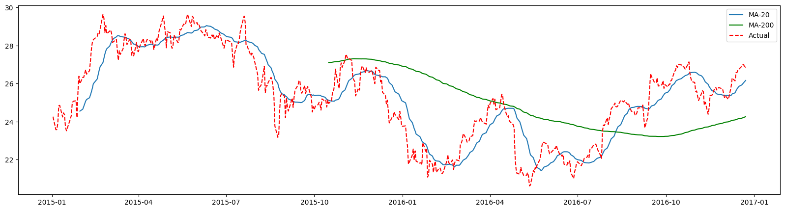
Comparison of Short and Long MA
Let’s compare the moving averages with window lengths of 20 and 200 for Apple stock closing values.
import yfinance as yf
START, END = '2015-1-1', '2020-12-31'
df = yf.Ticker('AAPL').history(start=START, end=END)
df.head()
If the code above does not work due to a YFRateLimitError, you can load the data from the following URL using the pandas read_csv() method.
import pandas as pd
df = pd.read_csv('https://raw.githubusercontent.com/datasmp/datasets/refs/heads/main/apple_stock_data_raw.csv',
                parse_dates = ['Date'])
df['Date'] = pd.to_datetime(df['Date'], utc=True)
df.set_index('Date', inplace=True)
df.head()
| Open | High | Low | Close | Volume | Dividends | Stock Splits | |
|---|---|---|---|---|---|---|---|
| Date | |||||||
| 2015-01-02 05:00:00+00:00 | 24.718174 | 24.729270 | 23.821672 | 24.261047 | 212818400 | 0.0 | 0.0 |
| 2015-01-05 05:00:00+00:00 | 24.030267 | 24.110154 | 23.391177 | 23.577578 | 257142000 | 0.0 | 0.0 |
| 2015-01-06 05:00:00+00:00 | 23.641929 | 23.839426 | 23.218087 | 23.579796 | 263188400 | 0.0 | 0.0 |
| 2015-01-07 05:00:00+00:00 | 23.788380 | 24.010286 | 23.677426 | 23.910429 | 160423600 | 0.0 | 0.0 |
| 2015-01-08 05:00:00+00:00 | 24.238858 | 24.886824 | 24.121246 | 24.829128 | 237458000 | 0.0 | 0.0 |
df.reset_index(inplace=True)
df['Date'] = df.Date.dt.date
df.set_index('Date', inplace=True)
df.head().round(2)
| Open | High | Low | Close | Volume | Dividends | Stock Splits | |
|---|---|---|---|---|---|---|---|
| Date | |||||||
| 2015-01-02 | 24.72 | 24.73 | 23.82 | 24.26 | 212818400 | 0.0 | 0.0 |
| 2015-01-05 | 24.03 | 24.11 | 23.39 | 23.58 | 257142000 | 0.0 | 0.0 |
| 2015-01-06 | 23.64 | 23.84 | 23.22 | 23.58 | 263188400 | 0.0 | 0.0 |
| 2015-01-07 | 23.79 | 24.01 | 23.68 | 23.91 | 160423600 | 0.0 | 0.0 |
| 2015-01-08 | 24.24 | 24.89 | 24.12 | 24.83 | 237458000 | 0.0 | 0.0 |
import pandas as pd
df_sma = pd.DataFrame(df.Close)
df_sma.head()
| Close | |
|---|---|
| Date | |
| 2015-01-02 | 24.261047 |
| 2015-01-05 | 23.577578 |
| 2015-01-06 | 23.579796 |
| 2015-01-07 | 23.910429 |
| 2015-01-08 | 24.829128 |
df_sma['MA-2'] = df_sma.Close.rolling(2).mean()
df_sma.head()
| Close | MA-2 | |
|---|---|---|
| Date | ||
| 2015-01-02 | 24.261047 | NaN |
| 2015-01-05 | 23.577578 | 23.919312 |
| 2015-01-06 | 23.579796 | 23.578687 |
| 2015-01-07 | 23.910429 | 23.745112 |
| 2015-01-08 | 24.829128 | 24.369779 |
df_sma['MA-3'] = df_sma.Close.rolling(3).mean()
df_sma.head()
| Close | MA-2 | MA-3 | |
|---|---|---|---|
| Date | |||
| 2015-01-02 | 24.261047 | NaN | NaN |
| 2015-01-05 | 23.577578 | 23.919312 | NaN |
| 2015-01-06 | 23.579796 | 23.578687 | 23.806140 |
| 2015-01-07 | 23.910429 | 23.745112 | 23.689267 |
| 2015-01-08 | 24.829128 | 24.369779 | 24.106451 |
import matplotlib.pyplot as plt
plt.figure(figsize=(20,5))
N = 500
plt.plot(df_sma.Close.rolling(20).mean()[:N], label='MA-20')
plt.plot(df_sma.Close.rolling(200).mean()[:N], label='MA-200', c='g')
plt.plot(df_sma.Close[:N], 'r--',label='Actual')
plt.legend();
Exponential Moving Average#
In this type of moving average, the effect of the recent values is greater than that of the older values. This is done by assigning weights to each day; these weights are multiplied by the corresponding stock prices and divided by the sum of all weights. For the values 100,120,170, the ordinary average is \(\frac{100+120+170}{3}=130\) If we use the weights 2,3,5, then: \(\frac{100\times 2+ 120\times 3 + 170\times 5}{2+3+5} = \frac{1410}{10}=141\)
Since the weight for the most recent value (170) is larger, its effect is greater, and the exponential moving average is larger than the regular moving average.
As a simple example, consider the stock prices in order: 100,110,90,105,95. If the period is chosen as 3 and the weights are 2,3,5, then for each 3 consecutive values the weighted moving average is computed as follows:
\(\displaystyle \frac{100\times 2+ 110\times 3 + 90\times 5}{2+3+5} = \frac{980}{10}=98\)
\(\displaystyle \frac{110\times 2+ 90\times 3 + 105\times 5}{2+3+5} = \frac{1015}{10}=101.5\)
\(\displaystyle \frac{90\times 2+ 105\times 3 + 95\times 5}{2+3+5} = \frac{970}{10}=97\)
In a pandas DataFrame, the ewm() method is used to calculate the exponential moving average. ewm stands for exponentially weighted moving average. For this function there is no fixed window size.
If the adjust parameter of the ewm() method is set to True, to calculate the exponentially weighted value at time step \(y_t\), all previous time step values \([x_0, x_1, ...,x_t]\) are used as follows:
\(\displaystyle y_t = \frac{x_t+(1-\alpha)x_{t-1}+(1-\alpha)^2x_{t-2}+...+(1-\alpha)^tx_{o}}{1+(1-\alpha)+(1-\alpha)^2+...+(1-\alpha)^{t-1}}\)
Thw weights are \(1, (1-\alpha), (1-\alpha)^2, ..., (1-\alpha)^{t-1}\) where \(\alpha\) is the smoothing factor between 0 and 1.
df_ewm = pd.DataFrame(df.Close)
df_ewm.head()
| Close | |
|---|---|
| Date | |
| 2015-01-02 | 24.261047 |
| 2015-01-05 | 23.577578 |
| 2015-01-06 | 23.579796 |
| 2015-01-07 | 23.910429 |
| 2015-01-08 | 24.829128 |
As \(\alpha\) gets closer to 1, the ewm values get closer to the actual values. Therefore, large alpha values correspond to shorter exponential moving averages, whereas small alpha values correspond to longer moving averages.
df_ewm['EWM_0_1'] = df_ewm.Close.ewm(alpha=0.3).mean()
df_ewm['EWM_0_5'] = df_ewm.Close.ewm(alpha=0.5).mean()
df_ewm['EWM_0_9'] = df_ewm.Close.ewm(alpha=0.9).mean()
df_ewm.head().round(2)
| Close | EWM_0_1 | EWM_0_5 | EWM_0_9 | |
|---|---|---|---|---|
| Date | ||||
| 2015-01-02 | 24.26 | 24.26 | 24.26 | 24.26 |
| 2015-01-05 | 23.58 | 23.86 | 23.81 | 23.64 |
| 2015-01-06 | 23.58 | 23.73 | 23.68 | 23.59 |
| 2015-01-07 | 23.91 | 23.80 | 23.80 | 23.88 |
| 2015-01-08 | 24.83 | 24.17 | 24.33 | 24.73 |
plt.figure(figsize=(20,5))
N = 10
plt.plot(df_ewm['EWM_0_1'][:N], label='EWM_0_1')
plt.plot(df_ewm['EWM_0_5'][:N], label='EWM_0_5')
plt.plot(df_ewm['EWM_0_9'][:N], label='EWM_0_9')
plt.plot(df_ewm.Close[:N], 'r--',label='Actual')
plt.legend();

Moving Average Convergence Divergence#
Moving Average Convergence Divergence (MACD) is the difference between the shorter exponential moving average and the longer one. It is common to choose 12 and 26 day EMA. You can use the span parameter of the ewm() method to get larger and smaller alpha values.
\(\alpha = \displaystyle \frac{2}{1+span}\)
Large span –> smaller \(\alpha\) –> slower decay –> EWM becomes smoother (longer-term average)
Small span –> larger \(\alpha\) –> fast decay –> EWM reacts more to recent data (short-term average)
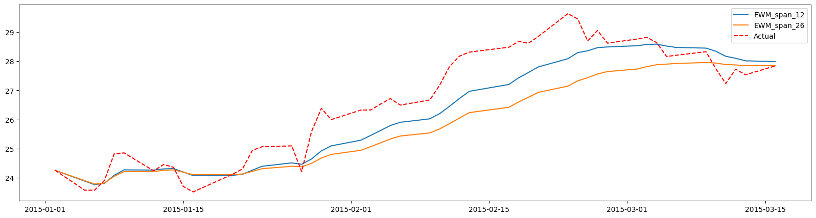
Let’s choose span values 12 and 26.
df_macd = pd.DataFrame(df.Close)
df_macd.head()
| Close | |
|---|---|
| Date | |
| 2015-01-02 | 24.261047 |
| 2015-01-05 | 23.577578 |
| 2015-01-06 | 23.579796 |
| 2015-01-07 | 23.910429 |
| 2015-01-08 | 24.829128 |
df_macd['EWM_span_12'] = df_macd.Close.ewm(span=12).mean()
df_macd['EWM_span_26'] = df_macd.Close.ewm(span=26).mean()
df_macd.head().round(2)
| Close | EWM_span_12 | EWM_span_26 | |
|---|---|---|---|
| Date | |||
| 2015-01-02 | 24.26 | 24.26 | 24.26 |
| 2015-01-05 | 23.58 | 23.89 | 23.91 |
| 2015-01-06 | 23.58 | 23.77 | 23.79 |
| 2015-01-07 | 23.91 | 23.81 | 23.82 |
| 2015-01-08 | 24.83 | 24.09 | 24.06 |
plt.figure(figsize=(20,5))
N = 50
plt.plot(df_macd['EWM_span_12'][:N], label='EWM_span_12')
plt.plot(df_macd['EWM_span_26'][:N], label='EWM_span_26')
plt.plot(df_macd.Close[:N], 'r--',label='Actual')
plt.legend();
df_macd['MACD_12_16'] = df_macd['EWM_span_12'] - df_macd['EWM_span_26']
df_macd.head()
| Close | EWM_span_12 | EWM_span_26 | MACD_12_16 | |
|---|---|---|---|---|
| Date | ||||
| 2015-01-02 | 24.261047 | 24.261047 | 24.261047 | 0.000000 |
| 2015-01-05 | 23.577578 | 23.890835 | 23.906169 | -0.015334 |
| 2015-01-06 | 23.579796 | 23.769436 | 23.788906 | -0.019470 |
| 2015-01-07 | 23.910429 | 23.813942 | 23.822879 | -0.008937 |
| 2015-01-08 | 24.829128 | 24.089765 | 24.056232 | 0.033532 |
Relative Strength Index#
Relative Strength Index (RSI) measures how strongly a stock’s price has moved in recent periods. It helps identify whether a stock is overbought or oversold. RSI value is between 0 and 100.
RSI > 70: Overbought RSI < 30: Oversold
Overbought means the price of the stock has increased too quickly or too much compared to its recent movement. This indicates unusually strong buying pressure, and a price correction (pullback) could happen soon.
Oversold means the price of the stock has decreased too quickly or too much compared to its recent movement. This indicates unusually strong selling pressure, and a price correction (pullback) could happen soon.
\(\displaystyle RSI = 100-\frac{100}{1+RS}\) where \(\displaystyle RS=\frac{Average\,\,gain\,\,over\,\,a\,\,period}{Average\,\,loss\,\,over\,\,a\,\,period}\) is the Relative strength
It is very common to choose a period of 14.
df_rsi = pd.DataFrame(df.Close)
df_rsi.head()
| Close | |
|---|---|
| Date | |
| 2015-01-02 | 24.261047 |
| 2015-01-05 | 23.577578 |
| 2015-01-06 | 23.579796 |
| 2015-01-07 | 23.910429 |
| 2015-01-08 | 24.829128 |
df_rsi['diff'] = df_rsi.diff()
df_rsi.head()
| Close | diff | |
|---|---|---|
| Date | ||
| 2015-01-02 | 24.261047 | NaN |
| 2015-01-05 | 23.577578 | -0.683470 |
| 2015-01-06 | 23.579796 | 0.002218 |
| 2015-01-07 | 23.910429 | 0.330633 |
| 2015-01-08 | 24.829128 | 0.918699 |
import numpy as np

df_rsi['gain'] =  np.where(df_rsi['diff']>0, df_rsi['diff'], 0)
df_rsi['loss'] = -np.where(df_rsi['diff']<0, df_rsi['diff'], 0)
df_rsi.head()
| Close | diff | gain | loss | |
|---|---|---|---|---|
| Date | ||||
| 2015-01-02 | 24.261047 | NaN | 0.000000 | -0.00000 |
| 2015-01-05 | 23.577578 | -0.683470 | 0.000000 | 0.68347 |
| 2015-01-06 | 23.579796 | 0.002218 | 0.002218 | -0.00000 |
| 2015-01-07 | 23.910429 | 0.330633 | 0.330633 | -0.00000 |
| 2015-01-08 | 24.829128 | 0.918699 | 0.918699 | -0.00000 |
df_rsi['gain_average_14'] =  df_rsi['gain'].rolling(14).mean()
df_rsi['loss_average_14'] =  df_rsi['loss'].rolling(14).mean()
df_rsi.iloc[10:15]
| Close | diff | gain | loss | gain_average_14 | loss_average_14 | |
|---|---|---|---|---|---|---|
| Date | ||||||
| 2015-01-16 | 23.519882 | -0.184181 | 0.000000 | 0.184181 | NaN | NaN |
| 2015-01-20 | 24.125687 | 0.605804 | 0.605804 | -0.000000 | NaN | NaN |
| 2015-01-21 | 24.309868 | 0.184181 | 0.184181 | -0.000000 | NaN | NaN |
| 2015-01-22 | 24.942297 | 0.632429 | 0.632429 | -0.000000 | 0.208274 | 0.159613 |
| 2015-01-23 | 25.071005 | 0.128708 | 0.128708 | -0.000000 | 0.217467 | 0.159613 |
RS = df_rsi['gain_average_14']/df_rsi['loss_average_14']
df_rsi['RSI'] =  100-(100/(1+RS))
df_rsi.iloc[10:15]
| Close | diff | gain | loss | gain_average_14 | loss_average_14 | RSI | |
|---|---|---|---|---|---|---|---|
| Date | |||||||
| 2015-01-16 | 23.519882 | -0.184181 | 0.000000 | 0.184181 | NaN | NaN | NaN |
| 2015-01-20 | 24.125687 | 0.605804 | 0.605804 | -0.000000 | NaN | NaN | NaN |
| 2015-01-21 | 24.309868 | 0.184181 | 0.184181 | -0.000000 | NaN | NaN | NaN |
| 2015-01-22 | 24.942297 | 0.632429 | 0.632429 | -0.000000 | 0.208274 | 0.159613 | 56.613540 |
| 2015-01-23 | 25.071005 | 0.128708 | 0.128708 | -0.000000 | 0.217467 | 0.159613 | 57.671326 |
plt.figure(figsize=(20,5))
N = 150
plt.plot(df_rsi['RSI'][:N])
plt.hlines(70, df_rsi.index[0], df_rsi.index[N-1], color='red', linestyle='--')
plt.hlines(30, df_rsi.index[0], df_rsi.index[N-1], color='green', linestyle='--')
plt.title('Relative Strength Index (RSI)');

Let’s combine the steps for building the RSI data into a single function for use in later applications.
def rsi_func(close_data):
    df_temp = pd.DataFrame(close_data)
    df_temp['diff'] = df_temp.diff()
    df_temp['gain'] =  np.where(df_temp['diff']>0, df_temp['diff'], 0)
    df_temp['loss'] = -np.where(df_temp['diff']<0, df_temp['diff'], 0)
    df_temp['gain_average_14'] =  df_temp['gain'].rolling(14).mean()
    df_temp['loss_average_14'] =  df_temp['loss'].rolling(14).mean()
    rs = df_temp['gain_average_14']/df_temp['loss_average_14']
    return  100-(100/(1+rs))


rsi_func(df.Close).tail()
Date
2020-12-23    67.006050
2020-12-24    70.334759
2020-12-28    73.856972
2020-12-29    68.526986
2020-12-30    72.226512
dtype: float64
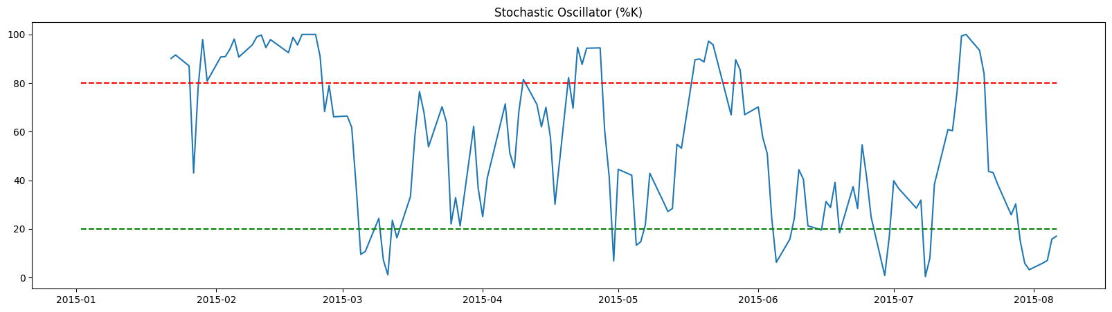
Stochastic Oscillator#
The Stochastic Oscillator (SO) is a commonly used momentum indicator that compares the closing price to the price range over a chosen period, typically 14. The SO value ranges between 0 and 100.
SO > 80: Overbought
SO < 20: Oversold
The notation used for the Stochastic Oscillator is %K, and its formula is as follows:
\(\displaystyle \%K = \frac{Close\, -\, Low_{N} }{High_{N}\, -\, Low_{N}}\times 100\)
where \(N\) represents the period, \(Low_{N}\) is the lowest price over the last \(N\) periods, and \(High_{N}\) is the highest price over the last \(N\) periods.
df_so = pd.DataFrame(df[['Close', 'High', 'Low']])
df_so.head()
| Close | High | Low | |
|---|---|---|---|
| Date | |||
| 2015-01-02 | 24.261047 | 24.729270 | 23.821672 |
| 2015-01-05 | 23.577578 | 24.110154 | 23.391177 |
| 2015-01-06 | 23.579796 | 23.839426 | 23.218087 |
| 2015-01-07 | 23.910429 | 24.010286 | 23.677426 |
| 2015-01-08 | 24.829128 | 24.886824 | 24.121246 |
df_so['Low_14'] = df_so.Low.rolling(14).min()
df_so['High_14'] = df_so.High.rolling(14).max()
df_so['%K'] = (df.Close-df_so['Low_14'])/(df_so['High_14']-df_so['Low_14'])*100
df_so.tail()
| Close | High | Low | Low_14 | High_14 | %K | |
|---|---|---|---|---|---|---|
| Date | ||||||
| 2020-12-23 | 127.606926 | 129.039275 | 127.431527 | 117.073677 | 130.968562 | 75.806665 |
| 2020-12-24 | 128.591034 | 130.042889 | 127.743314 | 117.073677 | 130.968562 | 82.889184 |
| 2020-12-28 | 133.190170 | 133.823522 | 130.091584 | 117.073677 | 133.823522 | 96.218763 |
| 2020-12-29 | 131.416748 | 135.236378 | 130.900319 | 117.073677 | 135.236378 | 78.969926 |
| 2020-12-30 | 130.296249 | 132.508133 | 129.984435 | 117.073677 | 135.236378 | 72.800696 |
plt.figure(figsize=(20,5))
N = 150
plt.plot(df_so['%K'][:N])
plt.hlines(80, df_rsi.index[0], df_rsi.index[N-1], color='red', linestyle='--')
plt.hlines(20, df_rsi.index[0], df_rsi.index[N-1], color='green', linestyle='--')
plt.title('Stochastic Oscillator (%K)');
Let’s combine the steps for building the RSI data into a single function for use in later applications.
def so_func(df_data):
    df_temp = pd.DataFrame(df_data[['Close', 'High', 'Low']])
    df_temp['Low_14'] = df_temp.Low.rolling(14).min()
    df_temp['High_14'] = df_temp.High.rolling(14).max()
    return (df_data.Close-df_temp['Low_14'])/(df_temp['High_14']-df_temp['Low_14'])*100


so_func(df).tail()
Date
2020-12-23    75.806665
2020-12-24    82.889184
2020-12-28    96.218763
2020-12-29    78.969926
2020-12-30    72.800696
dtype: float64
Commodity Channel Index#
The Commodity Channel Index (CCI) is a momentum indicator that shows the difference of the price of the stock from its center in terms of average deviation.
The CCI value ranges mostly but not always between -100 and 100.
CCI > 100: overbought
CCI < -100: oversold
The following is the standard formula for CCI: \(\displaystyle CCI = \frac{Typical\,Price - SMA(Typical\,Price)}{0.015\times MD(Typical\,Price)}\)
where
\(\displaystyle Typical\,Price = \frac{High\,+\,Low\,+\,Close}{3}\)
\(SMA\) is the simple moving average over \(N\) periods
\(MD\) is the mean absolute deviation over \(N\) periods:
\(\displaystyle MD = \frac{1}{N} \sum_{i=1}^N |Typical\,Price_i - SMA(Typical\,Price)_N|\).
df_cci = pd.DataFrame(df[['Close', 'High', 'Low']])
df_cci.head()
| Close | High | Low | |
|---|---|---|---|
| Date | |||
| 2015-01-02 | 24.261047 | 24.729270 | 23.821672 |
| 2015-01-05 | 23.577578 | 24.110154 | 23.391177 |
| 2015-01-06 | 23.579796 | 23.839426 | 23.218087 |
| 2015-01-07 | 23.910429 | 24.010286 | 23.677426 |
| 2015-01-08 | 24.829128 | 24.886824 | 24.121246 |
df_cci['TP'] = (df_cci['High'] + df_cci['Low'] + df_cci['Close']) / 3
df_cci['SMA_TP'] = df_cci['TP'].rolling(20).mean()
df_cci['MD']  = df_cci['TP'].rolling(20).apply(lambda x: abs(x - x.mean()).mean())
df_cci['CCI'] = (df_cci['TP']-df_cci['SMA_TP'])/(0.015*df_cci['MD'])
df_cci.tail()
| Close | High | Low | TP | SMA_TP | MD | CCI | |
|---|---|---|---|---|---|---|---|
| Date | |||||||
| 2020-12-23 | 127.606926 | 129.039275 | 127.431527 | 128.025909 | 120.768748 | 3.208622 | 150.784578 |
| 2020-12-24 | 128.591034 | 130.042889 | 127.743314 | 128.792412 | 121.557684 | 3.359588 | 143.563792 |
| 2020-12-28 | 133.190170 | 133.823522 | 130.091584 | 132.368425 | 122.487256 | 3.604047 | 182.779124 |
| 2020-12-29 | 131.416748 | 135.236378 | 130.900319 | 132.517815 | 123.318253 | 3.776107 | 162.417064 |
| 2020-12-30 | 130.296249 | 132.508133 | 129.984435 | 130.929606 | 123.917670 | 3.979971 | 117.453725 |
plt.figure(figsize=(20,5))
N = 150
plt.plot(df_cci['CCI'][:N])
plt.hlines(100, df_cci.index[0], df_cci.index[N-1], color='red', linestyle='--')
plt.hlines(-100, df_cci.index[0], df_cci.index[N-1], color='green', linestyle='--')
plt.title('Commodity Channel Index (CCI)');

Let’s combine the steps for building the RSI data into a single function for use in later applications.
def cci_func(df_data):
    df_temp = pd.DataFrame(df_data[['Close', 'High', 'Low']])
    df_temp['TP'] = (df_temp['High'] + df_temp['Low'] + df_temp['Close']) / 3
    df_temp['SMA_TP'] = df_temp['TP'].rolling(20).mean()
    df_temp['MD']  = df_temp['TP'].rolling(20).apply(lambda x: abs(x - x.mean()).mean())
    return (df_temp['TP']-df_temp['SMA_TP'])/(0.015*df_temp['MD'])

cci_func(df).tail()
Date
2020-12-23    150.784578
2020-12-24    143.563792
2020-12-28    182.779124
2020-12-29    162.417064
2020-12-30    117.453725
dtype: float64
Data Preparation#
Combined Data#
First, we will store all technical indicators and closing prices in a single DataFrame.
df.head()
| Open | High | Low | Close | Volume | Dividends | Stock Splits | |
|---|---|---|---|---|---|---|---|
| Date | |||||||
| 2015-01-02 | 24.718174 | 24.729270 | 23.821672 | 24.261047 | 212818400 | 0.0 | 0.0 |
| 2015-01-05 | 24.030267 | 24.110154 | 23.391177 | 23.577578 | 257142000 | 0.0 | 0.0 |
| 2015-01-06 | 23.641929 | 23.839426 | 23.218087 | 23.579796 | 263188400 | 0.0 | 0.0 |
| 2015-01-07 | 23.788380 | 24.010286 | 23.677426 | 23.910429 | 160423600 | 0.0 | 0.0 |
| 2015-01-08 | 24.238858 | 24.886824 | 24.121246 | 24.829128 | 237458000 | 0.0 | 0.0 |
data = pd.DataFrame(df.Close)
data.head()
| Close | |
|---|---|
| Date | |
| 2015-01-02 | 24.261047 |
| 2015-01-05 | 23.577578 |
| 2015-01-06 | 23.579796 |
| 2015-01-07 | 23.910429 |
| 2015-01-08 | 24.829128 |
data['sma'] = df.Close.rolling(10).mean()
data.tail()
| Close | sma | |
|---|---|---|
| Date | ||
| 2020-12-23 | 127.606926 | 123.704443 |
| 2020-12-24 | 128.591034 | 124.555090 |
| 2020-12-28 | 133.190170 | 125.946525 |
| 2020-12-29 | 131.416748 | 127.222006 |
| 2020-12-30 | 130.296249 | 127.791058 |
data['ewa'] = df_ewm.Close.ewm(alpha=0.3).mean()
data.tail().round(2)
| Close | sma | ewa | |
|---|---|---|---|
| Date | |||
| 2020-12-23 | 127.61 | 123.70 | 125.86 |
| 2020-12-24 | 128.59 | 124.56 | 126.68 |
| 2020-12-28 | 133.19 | 125.95 | 128.63 |
| 2020-12-29 | 131.42 | 127.22 | 129.47 |
| 2020-12-30 | 130.30 | 127.79 | 129.72 |
data['macd'] = df_macd.Close.ewm(span=12).mean() - df_macd.Close.ewm(span=26).mean()
data.tail().round(2)
| Close | sma | ewa | macd | |
|---|---|---|---|---|
| Date | ||||
| 2020-12-23 | 127.61 | 123.70 | 125.86 | 3.09 |
| 2020-12-24 | 128.59 | 124.56 | 126.68 | 3.25 |
| 2020-12-28 | 133.19 | 125.95 | 128.63 | 3.71 |
| 2020-12-29 | 131.42 | 127.22 | 129.47 | 3.89 |
| 2020-12-30 | 130.30 | 127.79 | 129.72 | 3.89 |
data['rsi'] = rsi_func(df.Close)
data.tail().round(2)
| Close | sma | ewa | macd | rsi | |
|---|---|---|---|---|---|
| Date | |||||
| 2020-12-23 | 127.61 | 123.70 | 125.86 | 3.09 | 67.01 |
| 2020-12-24 | 128.59 | 124.56 | 126.68 | 3.25 | 70.33 |
| 2020-12-28 | 133.19 | 125.95 | 128.63 | 3.71 | 73.86 |
| 2020-12-29 | 131.42 | 127.22 | 129.47 | 3.89 | 68.53 |
| 2020-12-30 | 130.30 | 127.79 | 129.72 | 3.89 | 72.23 |
data['so'] = so_func(df)
data.tail().round(2)
| Close | sma | ewa | macd | rsi | so | |
|---|---|---|---|---|---|---|
| Date | ||||||
| 2020-12-23 | 127.61 | 123.70 | 125.86 | 3.09 | 67.01 | 75.81 |
| 2020-12-24 | 128.59 | 124.56 | 126.68 | 3.25 | 70.33 | 82.89 |
| 2020-12-28 | 133.19 | 125.95 | 128.63 | 3.71 | 73.86 | 96.22 |
| 2020-12-29 | 131.42 | 127.22 | 129.47 | 3.89 | 68.53 | 78.97 |
| 2020-12-30 | 130.30 | 127.79 | 129.72 | 3.89 | 72.23 | 72.80 |
data['cci'] = cci_func(df)
data.tail().round(2)
| Close | sma | ewa | macd | rsi | so | cci | |
|---|---|---|---|---|---|---|---|
| Date | |||||||
| 2020-12-23 | 127.61 | 123.70 | 125.86 | 3.09 | 67.01 | 75.81 | 150.78 |
| 2020-12-24 | 128.59 | 124.56 | 126.68 | 3.25 | 70.33 | 82.89 | 143.56 |
| 2020-12-28 | 133.19 | 125.95 | 128.63 | 3.71 | 73.86 | 96.22 | 182.78 |
| 2020-12-29 | 131.42 | 127.22 | 129.47 | 3.89 | 68.53 | 78.97 | 162.42 |
| 2020-12-30 | 130.30 | 127.79 | 129.72 | 3.89 | 72.23 | 72.80 | 117.45 |
We will use the log return values of the close price, so let’s update the Close column.
data.Close = np.log(df.Close/df.Close.shift(1))
data.head()
| Close | sma | ewa | macd | rsi | so | cci | |
|---|---|---|---|---|---|---|---|
| Date | |||||||
| 2015-01-02 | NaN | NaN | 24.261047 | 0.000000 | NaN | NaN | NaN |
| 2015-01-05 | -0.028576 | NaN | 23.859006 | -0.015334 | NaN | NaN | NaN |
| 2015-01-06 | 0.000094 | NaN | 23.731513 | -0.019470 | NaN | NaN | NaN |
| 2015-01-07 | 0.013924 | NaN | 23.802147 | -0.008937 | NaN | NaN | NaN |
| 2015-01-08 | 0.037703 | NaN | 24.172484 | 0.033532 | NaN | NaN | NaN |
data.dropna(inplace = True)
data.head().round(2)
| Close | sma | ewa | macd | rsi | so | cci | |
|---|---|---|---|---|---|---|---|
| Date | |||||||
| 2015-01-30 | -0.01 | 24.93 | 25.53 | 0.29 | 58.43 | 80.81 | 181.75 |
| 2015-02-02 | 0.01 | 25.21 | 25.77 | 0.35 | 66.04 | 90.74 | 149.62 |
| 2015-02-03 | 0.00 | 25.43 | 25.94 | 0.38 | 64.90 | 90.88 | 137.34 |
| 2015-02-04 | 0.01 | 25.65 | 26.12 | 0.42 | 66.96 | 93.79 | 134.84 |
| 2015-02-05 | 0.01 | 25.83 | 26.30 | 0.46 | 75.50 | 98.12 | 129.30 |
Lagged Data#
def lag_func(data, name, lag):
    df_lag = pd.DataFrame(data[name])
    for i in range(1, lag+1):
        df_lag[f'lag_{i}'] = df_lag[name].shift(i)
        df_lag.dropna(inplace=True)
    return df_lag
lag_func(data, name='Close', lag=10).head().round(3)
| Close | lag_1 | lag_2 | lag_3 | lag_4 | lag_5 | lag_6 | lag_7 | lag_8 | lag_9 | lag_10 | |
|---|---|---|---|---|---|---|---|---|---|---|---|
| Date | |||||||||||
| 2015-04-21 | -0.005 | 0.023 | -0.011 | -0.005 | 0.004 | -0.004 | -0.002 | 0.004 | 0.008 | -0.003 | -0.011 |
| 2015-04-22 | 0.013 | -0.005 | 0.023 | -0.011 | -0.005 | 0.004 | -0.004 | -0.002 | 0.004 | 0.008 | -0.003 |
| 2015-04-23 | 0.008 | 0.013 | -0.005 | 0.023 | -0.011 | -0.005 | 0.004 | -0.004 | -0.002 | 0.004 | 0.008 |
| 2015-04-24 | 0.005 | 0.008 | 0.013 | -0.005 | 0.023 | -0.011 | -0.005 | 0.004 | -0.004 | -0.002 | 0.004 |
| 2015-04-27 | 0.018 | 0.005 | 0.008 | 0.013 | -0.005 | 0.023 | -0.011 | -0.005 | 0.004 | -0.004 | -0.002 |
Now we will define a dictionary that stores a DataFrame for each column in the data DataFrame, containing their lagged values.
df_dict = {}
for col in data.columns:
    df_dict[col] =  lag_func(data, name=col, lag=10)
df_dict['rsi'].head().round(2)
| rsi | lag_1 | lag_2 | lag_3 | lag_4 | lag_5 | lag_6 | lag_7 | lag_8 | lag_9 | lag_10 | |
|---|---|---|---|---|---|---|---|---|---|---|---|
| Date | |||||||||||
| 2015-04-21 | 59.27 | 54.20 | 55.03 | 56.67 | 61.55 | 48.89 | 48.97 | 53.23 | 47.61 | 42.70 | 47.51 |
| 2015-04-22 | 64.65 | 59.27 | 54.20 | 55.03 | 56.67 | 61.55 | 48.89 | 48.97 | 53.23 | 47.61 | 42.70 |
| 2015-04-23 | 64.61 | 64.65 | 59.27 | 54.20 | 55.03 | 56.67 | 61.55 | 48.89 | 48.97 | 53.23 | 47.61 |
| 2015-04-24 | 60.88 | 64.61 | 64.65 | 59.27 | 54.20 | 55.03 | 56.67 | 61.55 | 48.89 | 48.97 | 53.23 |
| 2015-04-27 | 72.90 | 60.88 | 64.61 | 64.65 | 59.27 | 54.20 | 55.03 | 56.67 | 61.55 | 48.89 | 48.97 |
Output Data#
The following outputs are defined for the regression and classification tasks. For the classification task, the classes are determined based on whether the log return of the closing price is positive. A class label of +1 indicates that the price increases, while 0 indicates non-increasing behavior (either a decrease or no change).
yR = df_dict['Close'].Close.values
yR.shape
(1436,)
yC = np.where(yR > 0, 1, 0)
yC.shape
(1436,)
Input Data#
We will generate a three-dimensional dataset as input for the LSTM model.
For each day, we have a sequence of length 10 for each of the 8 features (past values of the closing price and technical indicators).
X = df_dict['Close'].iloc[:,1:].values
X = X.reshape(X.shape+(1,))
X.shape
(1436, 10, 1)
for col in data.columns[1:]:
    new_input = df_dict[col].iloc[:,1:].values
    new_input = new_input.reshape(new_input.shape+(1,))
    X = np.concatenate([X, new_input], axis=2)

X.shape
(1436, 10, 7)
Split Data#
N = X.shape[0] # total number of rows

tr = 0.90 # train ratio
vr = (1-tr)/2 # validation ratio

ts = int(N*tr) # training size
vs = int(N*vr) # validation size

X_train, yR_train, yC_train = X[:ts], yR[:ts], yC[:ts]
X_valid, yR_valid, yC_valid = X[ts:ts+vs], yR[ts:ts+vs], yC[ts:ts+vs]
X_test , yR_test , yC_test  = X[ts+vs:], yR[ts+vs:], yC[ts+vs:]
X_train.shape, yR_train.shape, yC_train.shape
((1292, 10, 7), (1292,), (1292,))
X_valid.shape, yR_valid.shape, yC_valid.shape
((71, 10, 7), (71,), (71,))
X_test.shape, yR_test.shape, yC_test.shape
((73, 10, 7), (73,), (73,))
LSTM#
from tensorflow import keras
model = keras.models.Sequential([
    keras.layers.Input((None, 8)),
    keras.layers.LSTM(100, activation='relu', return_sequences=True),
    keras.layers.LSTM(200, activation='relu'),
    keras.layers.Dense(1, activation='sigmoid')])
model.summary()
Model: "sequential"
┏━━━━━━━━━━━━━━━━━━━━━━━━━━━━━━━━━┳━━━━━━━━━━━━━━━━━━━━━━━━┳━━━━━━━━━━━━━━━┓
┃ Layer (type)                    ┃ Output Shape           ┃       Param # ┃
┡━━━━━━━━━━━━━━━━━━━━━━━━━━━━━━━━━╇━━━━━━━━━━━━━━━━━━━━━━━━╇━━━━━━━━━━━━━━━┩
│ lstm (LSTM)                     │ (None, None, 100)      │        43,600 │
├─────────────────────────────────┼────────────────────────┼───────────────┤
│ lstm_1 (LSTM)                   │ (None, 200)            │       240,800 │
├─────────────────────────────────┼────────────────────────┼───────────────┤
│ dense (Dense)                   │ (None, 1)              │           201 │
└─────────────────────────────────┴────────────────────────┴───────────────┘
Total params: 284,601 (1.09 MB)
Trainable params: 284,601 (1.09 MB)
Non-trainable params: 0 (0.00 B)
model.compile(loss='binary_crossentropy', metrics=['accuracy'])
model.fit(X_train, yC_train, validation_data=(X_valid, yC_valid))
---------------------------------------------------------------------------
ValueError                                Traceback (most recent call last)
Cell In[55], line 1
----> 1 model.fit(X_train, yC_train, validation_data=(X_valid, yC_valid))

File ~/anaconda3/lib/python3.11/site-packages/keras/src/utils/traceback_utils.py:122, in filter_traceback.<locals>.error_handler(*args, **kwargs)
    119     filtered_tb = _process_traceback_frames(e.__traceback__)
    120     # To get the full stack trace, call:
    121     # `keras.config.disable_traceback_filtering()`
--> 122     raise e.with_traceback(filtered_tb) from None
    123 finally:
    124     del filtered_tb

ValueError: Exception encountered when calling LSTMCell.call().

Dimensions must be equal, but are 7 and 8 for '{{node sequential_1/lstm_1/lstm_cell_1/MatMul}} = MatMul[T=DT_FLOAT, grad_a=false, grad_b=false, transpose_a=false, transpose_b=false](sequential_1/lstm_1/strided_slice_2, sequential_1/lstm_1/lstm_cell_1/Cast/ReadVariableOp)' with input shapes: [?,7], [8,400].

Arguments received by LSTMCell.call():
  • inputs=tf.Tensor(shape=(None, 7), dtype=float32)
  • states=('tf.Tensor(shape=(None, 100), dtype=float32)', 'tf.Tensor(shape=(None, 100), dtype=float32)')
  • training=True
model.predict(X_test[:5])
1/1 ━━━━━━━━━━━━━━━━━━━━ 0s 85ms/step
array([[0.8601803 ],
       [0.9889952 ],
       [0.9982691 ],
       [0.89139706],
       [0.9328328 ]], dtype=float32)
yC_test_pred = np.where(model.predict(X_test)>0.5, 1, 0)
yC_test_pred[:5]
3/3 ━━━━━━━━━━━━━━━━━━━━ 0s 5ms/step
array([[1],
       [1],
       [1],
       [1],
       [1]])
from sklearn.metrics import accuracy_score

accuracy_score(yC_test, yC_test_pred)
0.4794520547945205